
Named Arrays#
The Named Arrays page will contain a list of arrays saved in the Sitka session. it will look like this;
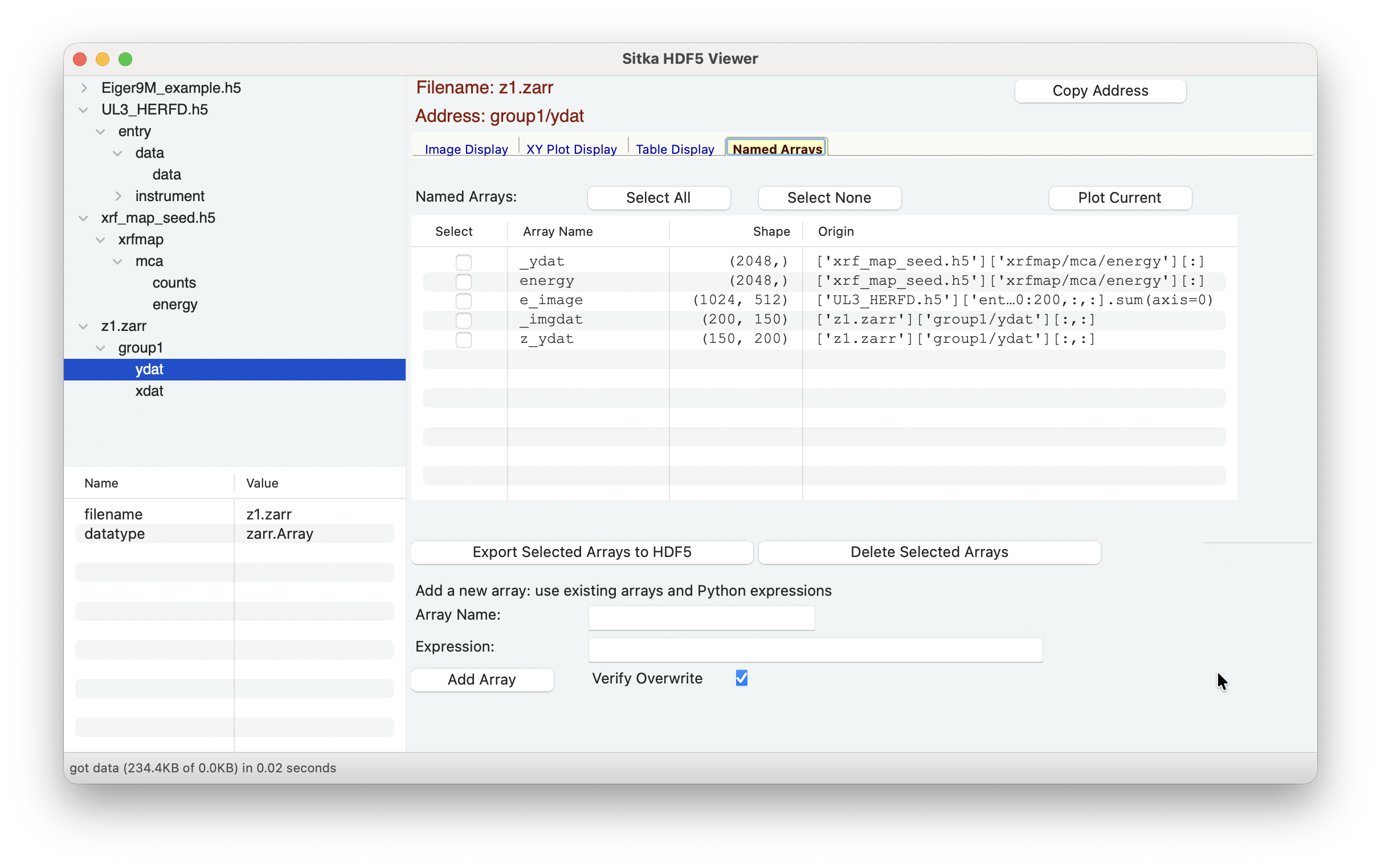
Each of the named Array can be highlighted, or multiple arrays can be selected at a time. The Plot Current button will show the highlighted array (as a simple plot or image display).
Note that this list may contain arrays named _imgdat, _ydat, and _tabledat. These arrays are automatically written as the last data used by the Image Display page, the XY Display page and the Table Display page.
You can use Delete Selected Arrays to remove selected named arrays.
You can also use the Export Selected Arrays to HDF5 to export
selected arrays to a simple HDF5 file. This will write the selected arrays
to a new HDF5 file, with all arrays put into a Group name sitka_arrays.
You can read this file in a later or different Sitka session. If you select
the sitka_arrays Group, the Import Named Arrays” at the upper right
of the main Sitka window will be enabled. Hitting that button will import
all of these named arrays into the Named Arrays panel. This allows you to
extract data from complex datasets and easily retrieve them for later analysis.
At the bottom of this page, you can also create a new array directly. Here you give a name (which must follow the valid conventions for a Python variable: A letter or underscore followed by any number of letters, numbers, or underscore), and an mathematical expression to evaluate for the array value. This uses an asteval Interpreter, which follows standard Python conventions for mathematical operations and array slicing, and includes many built-in math functions from the math module and numpy, and also contains the other named arrays. Example expressions include;
‘0.01 * arange(4096)’, maybe to set an X-axis for XYPlots
‘linspace(-2, 2, 501)’, as another form to set an X-axis for XYPlots
‘(image1 - image2)/image1.mean()’ to take a scaled difference of two images.
‘sin(ydat/10)’ - you can use any trig functions from numpy.
‘gradient(ydat)/gradient(xdat)’ to take the derivative ‘dy/dx’.
These calculated arrays can be used in the Image Display, XY Plot Display, and Table Display pages, and can be exported to HDF5 files for later use.