\(\newcommand{\AA}{\unicode{x212B}}\)
14.8. XAFS: Fitting XAFS to Feff Paths
Fitting XAFS data with structural models based on Feff calculations is a primary motivation for Larch. In this section, we describe how to set up a fitting model to fit a set of FEFF calculations to XAFS data. Many parts of the documentation so far have touched on important aspects of this process, and those sections will be referenced here.
14.8.1. The Feffit Strategy for Modeling EXAFS Data
The basic approach to modeling EXAFS data in Larch (see
[Newville (2001)b]) is to create a model EXAFS \(\chi(k)\) as a
sum of scattering path<s that will be compared to experimentally derived
\(\chi(k)\). The model will consist of a set of FEFF Scattering Paths
representing the photo-electron scattering from different sets of atoms.
As discussed in XAFS: Reading and using Feff Paths, these FEFF Paths have a fixed
set of physically meaningful parameters than can be modified to alter the
predicted contribution to \(\chi(k)\). Any of these values can be
defined as algebraic expressions of Larch Parameters defined by
_math.param(). The actual fit uses the same fitting infrastructure
as to _math.minimize() to refine the values of the variable
parameters in the model so as to best match the experimental data. Because
\(\chi(k)\) has known properties and \(k\) dependencies, it is
common to weight and Fourier transform (as described in XAFS: Fourier Transforms for XAFS)
for the analysis. In general term, the the refinement process will compare
experimental and model \(\chi(k)\) after a Transformation.
The model for \(\chi(k)\) used to compare to data is
where \(\chi_j\) is the EXAFS contribution for a FEFF Path, as given in
The EXAFS Equation using Feff and FeffPath Groups for path \(j\), where \(p_j\) is the
set of adjustable Path Parameters (\(S_0^2\), \(E_0\),
\(\delta{R}\), \(\sigma^2\), and so on) listed as Adjustable in
the Table of Feff Path Parameters.
The number of FEFF Paths used in the sum can be unlimited, and they do not need to originate from a single run of FEFF. This can be important in modeling even moderately complex structures as a single run of FEFF is limited to having exactly one absorbing atom in a cluster of atoms and therefore cannot be used to model multi-site systems without multiple runs.
Because a large number of FEFF Paths could be used to model an XAFS spectrum, and because each Feff Path has up to 8 adjustable parameters, there is the potential of having a very large number of parameters for a fit. In principle, However, there is a limited amount of information in an XAFS spectrum. A simple estimate of how many parameters could be independently measured is given from information theory of Shannon and Nyquist as
where \(\Delta k\) and \(\Delta R\) are the \(k\) and \(R\) range of the usable data under consideration. [Stern (1993)] argues convincingly that the ‘+1’ here should be ‘+2’, but we’ll remain conservative and keep the ‘+1’, and use this value not only for fit statistics but to limit the maximum number of free variables allowed in a fit. In general, this greatly limits the number of parameters thar can be successfully used in a fit. It should be noted that this limitation is inherent in XAFS (and many other techniques that rely on oscillatory signals), and not a consequence of using Fourier transforms in the analysis.
Because of this fundamental information limit, it is usual to purposely
limit the spectra being analyzed. Of course, one usually limits how far
out in energy to measure a signal based on the strength of the signal
compared to some noise level. This limits the \(k\) range of useful
data. In addition, the number of scattering paths that contribute to the
XAFS diverges very quickly with \(R\). For any \(R\) interval
then, the finite \(k\) range sets an upper limit on the number of
parameters available for describing the atomic partial pair distribution
function that gives spectral weight in that interval. The distance to
which a structural model can determined from real XAFS data is therefore
limited to 5 or so Angstroms. Because of these inherent limitations, it is
generally preferrable to analyze XAFS data by limiting the \(R\) range
of the analysis by using Fourier transforms to convert \(\chi(k)\) to
\(\chi(R)\). The feffit() function allows several choices of
data transformations, including doing 0 (\(k\), unfiltered), 1
(\(R\), or Fourier transformed), or 2 (math:q, or Fourier filtered)
Fourier transforms. Fitting in unfiltred \(k\) space is generally not
recommended.
14.8.2. Fit statistics and goodness-of-fit meassures for feffit()
The fit done by feffit() is conceptually very similar to the fits
described in minimize() and objective Functions. Therefore, many of the
statistics discussed in Fit Results and Outputs are also generated for
feffit(). In view of the limited amount of information, some of the
traditional statistical definitions need to be carefully examid, and
possibly altered slightly. For example, the typical \(\chi^2\)
statistic (as given in Fitting Overview) is
seems simple enough, but actually raises several questions, as we have to decide what each of the terms here is. As above, we’ll typically analyze data in \(R\) space after a Fourier transform, so that the “data” \(y\) actually represents the real and imaginary components of \(\chi(R)\), and the “model” \(f\) will also be the Fourier transform of the parameterized model for \(\chi(k)\).
Perhaps the largest questions are ones that are often dismissed as trivial in standard statistics discussions:
Perhaps surprisingly, the first question is: what is \(N\)? The \(\chi(k)\) data can be measured (or sampled) on an arbitrarily fine grid, and a Fourier transform can use an arbitrary number of points. Thus, the number of points for both \(\chi(k)\) and \(\chi(R)\) can easily be changed without actually changing the quality or quantity of the real data. The best number to use for the sum over the number of data points is then \(N_{\rm ind}\) defined above. Of course, we generally oversample the data, so the value for \(\chi^2\) used and reported is
where the sum can be over an arbitrary number of samples of \(\chi(k)\) or \(\chi(R)\), but the actual range of the data sets \(N_{\rm ind}\).
A second consideration is what to use for \(\epsilon\), the uncertainty
in the “data”. Of course, the uncertainty in the data, \(\epsilon\),
depends on the details of the data transformation (for example, whether
fitting in \(R\) or \(q\) space). Estimating the noise level in
any given spectrum is not at all trivial, and should generally involve a
proper statistical treatment of the data. For an individual spectrum, what
can be done easily and automatically is to estimate the noise level
assuming that the data is dominated by noise that is independent of
\(R\): white noise. The function estimate_noise() does this
[Newville, Boyanov, and Sayers (1999)], and the estimate derived from this method is
used unless you specify a value for epsilon_k the noise level in
\(\chi(k)\). Though usually \(\epsilon\) is taken to be a scalar
value, it can be specfied as an array (of the same length as
\(\chi(k)\)) if more accurate measures for the uncertainty of the data
is available.
It turns out that \(\chi^2\) is almost always too big, and reduced \(chi^2\) (that is, \(\chi^2/(p - N_{\rm ind})\) where \(p\) is the number of fitted parameters) is far greater than 1. This is partly due to a poor assessment of the uncertainty in the data, and partly due to imperfections in the calculations that go into the model. Together, these are often called “systematic errors” in the EXAFS literature. Because of this issue, an alternative statistic \(\cal{R}\) is often used as a supplement to \(\chi^2\) for EXAFS. The \(\cal{R}\) factor is defined as
which is to say, the misfit scaled by the magnitude of the data.
14.8.3. The Feffit functions in Larch
The function feffit() is the principle function to do the fit of a
set of Feff paths to XAFS spectra. This essentially runs
_math.minimize() with a parameter group holding all the variable and
constrained parameters, and with a built-in objective function to calculate
the fit residual. This objective function defines the residual as the
difference of model and experimental \(\chi(k)\) for a list of
Datasets. Here, a Feffit Dataset is an important concept that will
allow us to easily extend modeling to multiple data sets.
While conceptually fairly simple, the approach is quite general and
flexible, and the level of flexibility can sometimes be daunting. A
Feffit Dataset has three principle components. First, it has an
experimental data, \(\chi(k)\). Second, it has a list of Feff paths –
that will be used to calculate the model \(\chi(k)\) (using the same
calculation as used by ff2chi()). Third, it has a Feffit Transform
group which holds the Fourier transform and fitting ranges to select how
the data and model are to be compared. Since the fit is done with a single
group holding all the parameters, it is important that the Path Parameters
for all Feff Paths used in the fits should be written in terms of variable
parameters in a single parameter group.
There are then 3 principle functions for setting up and executing
feffit():
feffit_transform()is used to create a Transform group, which holds the set of Fourier transform parameters, fitting ranges, and space in which the data and sum of paths are to be compared.
feffit_dataset()is used to create a Dataset group, which consists of the three components described above:
a group holding experimental data (arrays holding
kandchi).a list of Feff paths.
a Transform group.
Finally,
feffit()is run with a parameter group containing the variable and constrained Parameters for the fit, and a dataset or list of datasets groups.
14.8.4. feffit_transform() and the Feffit Transform Group
- feffit_transform(fitspace='r', kmin=0, kmax=20, kweight=2, ...)
create and return Feffit Transform group to be used in a Feffit dataset.
- Parameters:
fitspace – name of FT type for fit: one of (‘k’, ‘r’, ‘q’, ‘w’), default ‘r’.
kmin – starting k for FT Window (0).
kmax – ending k for FT Window (20).
dk – tapering parameter for FT Window (4).
dk2 – second tapering parameter for FT Window (None).
window – name of window type (‘kaiser’).
nfft – value to use for \(N_{\rm fft}\) (2048).
kstep – value to use for \(\delta{k}\) (0.05).
kweight – exponent(s) for weighting spectra by \(k^{\rm kweight}\) (2).
rmin – starting R for Fit Range and/or reverse FT Window (0).
rmax – ending R for Fit Range and/or reverse FT Window (10).
dr – tapering parameter for reverse FT Window 0.
rwindow – name of window type for reverse FT Window (‘kaiser’).
- Returns:
a Feffit Transform group
The parameters stored in the returned Feffit Transform Group will be used to control how the fit is performed, including Fourier transform parameters and fit space for a fit. All the arguments passed in will be stored as variables of the same name in the Feffit Transform group. Additional variables may be stored in this group as well.
The returned Feffit Transform Group will have members listed in Feffit Transform Group Members.
Table of Feffit Transform Group Memebers Most of these parameters follow the conventions for
xftf()in section on Fourier Transforms for XAFS.
member name
description
fitspace
space used for fitting – one of
'k','r','q', or'w'('r')kmin
starting \(k\) for FT Window (0).
kmax
ending \(k\) for FT Window (20).
kweight
exponent(s) for weighting spectra by \(k^{\rm kweight}\) (2).
dk
tapering parameter for FT Window (4).
dk2
second tapering parameter for FT Window (
None– equal todk).window
name of window type for FT (
'kaiser').kstep
value to use for \(\delta{k}\) (0.05).
nfft
value to use for \(N_{\rm fft}\) (2048).
rmin
starting \(R\) for back FT Window (0).
rmax
ending \(R\) for back FT Window (10).
dr
tapering parameter for back FT Window (0).
dr2
second tapering parameter for back FT Window (
None– equal todr).rwindow
name of window type for back FT (
'hanning').
As an important note, kweight can either be a single integer value, or
a list or tuple of integers. Supplying more than one value will have the
effect of having all the kweights used in the fit. If multiple
\(k\) weights are provided, they can be in any order – kweight=(1,
2, 3) will produce the same result as kweight=(3, 1, 2). Some
functions (such as generating output arrays for plotting) may need to
assume 1 \(k\) weight – these will take the first one listed.
14.8.5. feffit_dataset()
- feffit_dataset(data=None, pathlist=[], transform=None)
create a Feffit Dataset group.
- param data:
group containing experimental EXAFS (needs arrays
kandchi).- param pathlist:
list of FeffPath groups, as created from
feffpath().- param transform:
Feffit Transform group.
- returns:
a Feffit Dataset group.
A Dataset group is pretty simple, initially consisting of sub-groups
data,pathlist, andtransform, though each of these can be complex.The value for
datamust be a group containing arrayskandchi(as determined_xafs.autobk()or some other procedure). If it contains a value (scalar or array)epsilon_k, that will be used as the uncertainty in \(\chi(k)\) for weighting the fit. Otherwise, the uncertainty in \(\chi(k)\) will be estimated automatically, and stored in this dataset.The
pathlistis a list of Feff Paths, each of which can have its Path Parameters written in terms of fit parameters (see the final example in the previous section). This list of paths will be sent toff2chi()to calculate the model \(\chi\) to compare to the experimental data. Finally,transformis a Feffit transform group, as defined above.A Dataset will also have a few other components, including:
component name
description
epsilon_k
estimated noise in the \(\chi(k)\) data.
epsilon_r
estimated noise in the \(\chi(R)\) data.
n_idp
estimated number of independent points in the data.
model
a group for the model \(\chi\) spectrum.
The
modelcomponent will be set after a fit, and will contain the standard set of arrays for \(\chi(k)\) and \(\chi(R)\) for the fitting model, and can be directly compared to the arrays for the experimental data.
14.8.6. feffit()
- feffit(paramgroup, datasets, rmax_out=10, path_outputs=True)
execute a Feffit fit.
- Parameters:
paramgroup – group containing parameters for fit
datasets – Feffit Dataset group or list of Feffit Dataset group.
rmax_out – maximum \(R\) value to calculate output arrays.
path_output – Flag to set whether all Path outputs should be written.
- Returns:
a fit results group.
The
paramgroupis a group containing all fitting parameters for the model. Thedatasetsargument can be either a single Feffit Dataset as created byfeffit_dataset()or a list of them. Ifpath_outputs==True, all Feff Paths in the fit will be separately Fourier transformed.When the fit is completed, the returned value will be a group containing three objects:
datasets: an array of FeffitDataSet groups used in the fit.params: This will be identical to the input parameter group.fit: an object which points to the low-level fit.
In addition, the output statistics listed below in Table of Feffit Output Statistics. will be written the
paramgroupgroup. Since each varied and constrained parameter will also have best-values and estimated uncertainties, this allows the parameter group to be considered the principle group for a particular fit – it holds the variable parameters and statistical results needed to compare two fits.On output, a new sub-group called
modelwill be created for each Feffit Dataset. This will parallel thedatagroup, in the sense that it will have output arrays listed in the Table of Feffit Output Arrays.If
path_outputs==True, all Feff Paths in the fit will be separately Fourier transformed., with the result being put in the corresponding FeffPath group.A final note on the outputs of
feffit(): theparamsub-group in the output is truly identical to the inputparamgroup. It is not a copy but points to the same group of values (see Object identities, copying, and equality vs. identity).
Table of Feffit Output Statistics. These values will be written to the
paramgroupgroup. Listed here are the group component name and a description of its content. Many of these are described in more detail in Fit Results and Outputs
component name
description
chi_reduced
reduced chi-square statistic.
chi_square
chi-square statistic.
covar
covariance matrix.
covar_vars
list of variable names for rows and columns of covariance matrix.
errorbars
Flag whether error bars could be calculated.
fit_details
group with additional fit details.
message
output message from fit.
nfree
number of degrees of freedom in fit.
nvarys
number of variables in fit.
Table of Feffit Output Arrays. The following arrays will be written into the
dataandmodelsub-group for each dataset. The arrays will be created using the Path Parameters used in the most recent fit and the Feffit Transform group. Many of these arrays have names following the conventions forxftf()in section on Fourier Transforms for XAFS.
array name
description
k
wavenumber array of \(k\).
chi
\(\chi(k)\).
kwin
window \(\Omega(k)\) (length of input chi(k)).
r
uniform array of \(R\), out to
rmax_out.chir
complex array of \(\tilde\chi(R)\).
chir_mag
magnitude of \(\tilde\chi(R)\).
chir_pha
phase of \(\tilde\chi(R)\).
chir_re
real part of \(\tilde\chi(R)\).
chir_im
imaginary part of \(\tilde\chi(R)\).
14.8.7. feffit_report()
14.8.8. Example 1: Simple fit with 1 Path
We start with a fairly minimal example, fitting spectra read from a data file with a single Feff Path.
## examples/feffit/doc_feffit1.lar

# import needed for python:
#from larch.io import read_ascii
#from larch.fitting import param, guess, param_group
#from larch.xafs import autobk, feffpath, feffit_transform, feffit_dataset, feffit, feffit_report
#from larch.wxlib.xafsplots import plot_chifit

# read data
cu_data  = read_ascii('../xafsdata/cu_metal_rt.xdi')
autobk(cu_data.energy, cu_data.mutrans, group=cu_data, rbkg=1.0, kw=2)

# define fitting parameter group
pars = param_group(amp    = param(1.0, vary=True),
                   del_e0 = param(0.0, vary=True),
                   sig2   = param(0.0, vary=True),
                   del_r  = guess(0.0, vary=True) )

# define a Feff Path, give expressions for Path Parameters
path1 = feffpath('feffcu01.dat',
                 s02    = 'amp',
                 e0     = 'del_e0',
                 sigma2 = 'sig2',
                 deltar = 'del_r')

# set tranform / fit ranges
trans = feffit_transform(kmin=3, kmax=17, kw=2, dk=4, window='kaiser', rmin=1.4, rmax=3.0)

# define dataset to include data, pathlist, transform
dset = feffit_dataset(data=cu_data, pathlist=[path1], transform=trans)

# perform fit!
out = feffit(pars, dset)
print(feffit_report(out))

try:
    fout = open('doc_feffit1.out', 'w')
    fout.write("%s\n" % feffit_report(out))
    fout.close()
except:
    print('could not write doc_feffit1.out')
#endtry
#
plot_chifit(dset)

## end examples/feffit/doc_feffit1.lar
This simply follows the essential steps:
1. A group of parameters
parsis defined. Note that you can include upper and/or lower bounds and mix the use of_math.guess()and_math.param().2. A Feff Path is defined with
feffpath(), as discussed in the previous section. Here we assign each of the Path Parameters to the name of one of the fitting parameters. More complex expressions and relations can be used, but for this example, we’re keeping it simple.3. A Feffit Transform is created with
feffit_transform(), which essentially sets the Fourier transform parameters and fit ranges.4. A Feffit Dataset is created with
feffit_dataset(). To begin the fit, this includes adatagroup, atransformgroup, and apathlist, which is a list of FeffPaths.5. The fit is run with
feffit(), and the output group is saved. This output group is used byfeffit_report()to generate a fit report (shown below).6. Plots are made from the dataset, using rather long-winded
plot()commands.
running this example prints out the following report:
=================== FEFFIT RESULTS ====================
[[Statistics]]
  n_function_calls     = 36
  n_variables          = 4
  n_data_points        = 104
  n_independent        = 15.2602829
  chi_square           = 112.726669
  reduced chi_square   = 10.0109979
  r-factor             = 0.00272181
  Akaike info crit     = 38.5161779
  Bayesian info crit   = 41.4171921

[[Variables]]
  amp                  =  0.9305631 +/- 0.0391214  (init= 1.0000000)
  del_e0               =  4.3577673 +/- 0.5113492  (init= 0.0000000)
  del_r                = -0.0060167 +/- 0.0026133  (init= 0.0000000)
  sig2                 =  0.0086697 +/- 3.0785e-4  (init= 0.0000000)

[[Correlations]] (unreported correlations are <  0.100)
  amp, sig2            =  0.928
  del_e0, del_r        =  0.920
  del_r, sig2          =  0.159
  amp, del_r           =  0.137

[[Dataset]]
  unique_id            = 'dmde5wld'
  fit space            = 'r'
  r-range              = 1.400, 3.000
  k-range              = 3.000, 17.000
  k window, dk         = 'kaiser', 4.000
  paths used in fit    = ['feffcu01.dat']
  k-weight             = 2
  epsilon_k            = Array(mean=6.1896e-4, std=0.0016546)
  epsilon_r            = 0.0208038
  n_independent        = 15.260

[[Paths]]
 = Path 'p3tf6mewg' = Cu K Edge
    feffdat file = feffcu01.dat, from feff run ''
    geometry  atom      x        y        z      ipot
              Cu       0.0000,  0.0000,  0.0000  0 (absorber)
              Cu       0.0000, -1.8016,  1.8016  1
     reff   =  2.5478000
     degen  =  12.000000
     n*s02  =  0.9305631 +/- 0.0391214  := 'amp'
     e0     =  4.3577673 +/- 0.5113492  := 'del_e0'
     r      =  2.5417833 +/- 0.0026133  := 'reff + del_r'
     deltar = -0.0060167 +/- 0.0026133  := 'del_r'
     sigma2 =  0.0086697 +/- 3.0785e-4  := 'sig2'

=======================================================
and generates the plots shown below
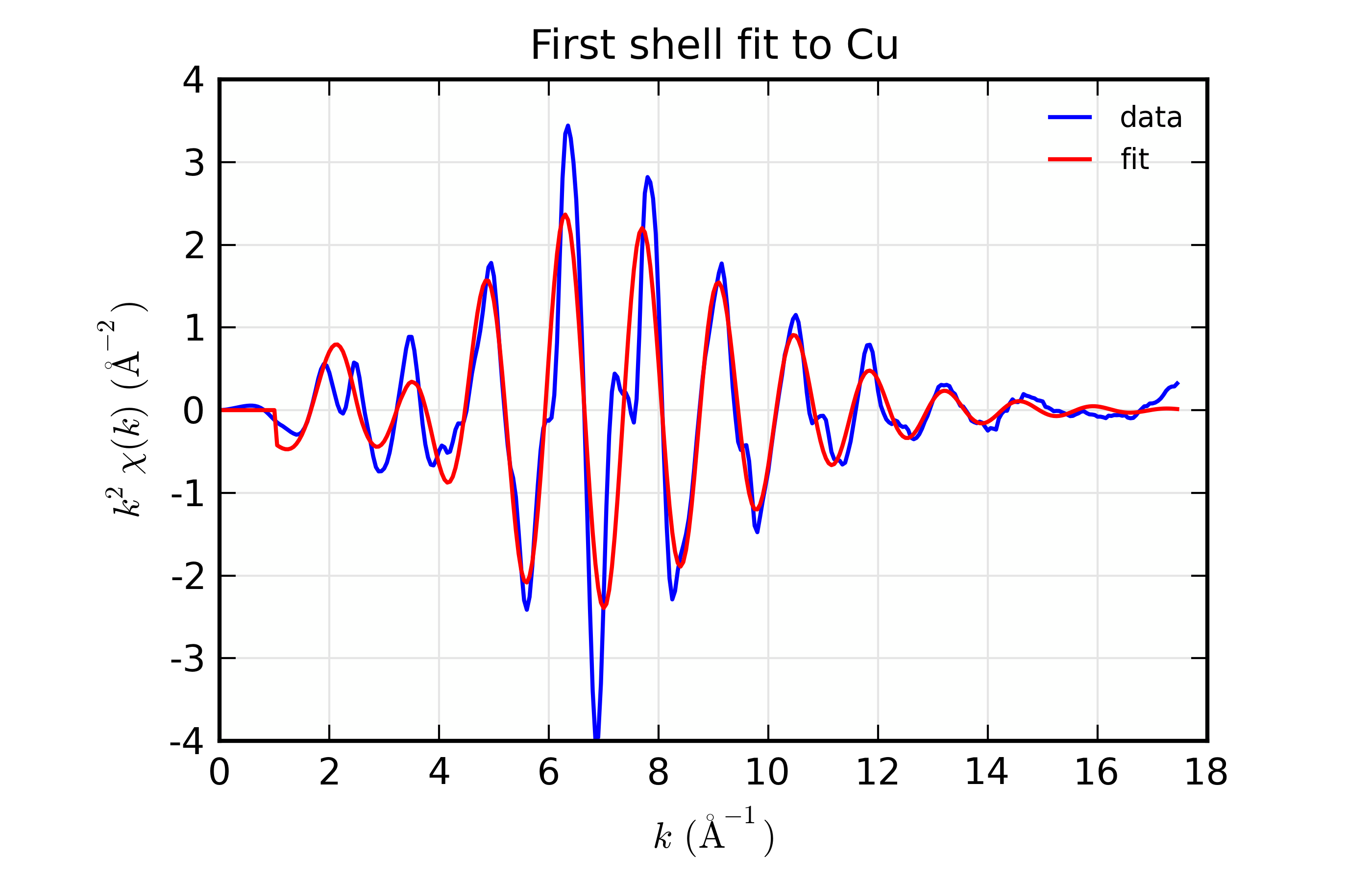 k space
 R space
Figure 14.8.8.1 Results for Feffit for a simple 1-shell fit to a spectrum from Cu metal. Left: Data and Fit in \(k\) space. Right: Data and Fit in \(R\) space
This is a pretty good fit to the first shell of Cu metal, and shows the basic mechanics of fitting XAFS data to Feff Paths. There are several things that might be added to this for modeling more complex XAFS data, including adding more paths to a fit, including multiple-scattering paths, simultaneously modeling more than one data set, and building more complex fitting models. We’ll get to these in the following examples.
But first, a small detour. The plotting commands in the above example for plotting \(\chi(k)\) and \(\chi(R)\) for data and model will be useful for the other examples as well, so we’ll create a slightly generalized function to make such plots and put this and several other plotting functions into a separate file, doc_macros.lar. This will look like this:
def write_report(filename, out):
    "write report to file"
    try:
        f = open(filename, 'w')
        f.write(out)
        f.close()
    except:
        print( 'could not write %s' % filename)
    #endtry
#enddef

## end of examples/feffit/doc_macros.lar
This defines several new plotting functions plot_chifit(),
plot_path_k(), and plot_path_r(), and so on which we’ll find
useful in later examples. Using the first of these, we can then replace
the plot commands in the script above with:
run('doc_macros.lar')
plot_chifit(dset, title='First shell fit to Cu')
and get reproducible plots without having to copy and paste the same code fragment everywhere. We’ll use this in the examples below.
14.8.9. Example 2: Fit 1 dataset with 3 Paths
We’ll continue with the Cu data set, and add more paths to model further shells. This is fairly straightforward, but in the interest of space, we’ll limit the example here to 3 paths to model the first two shells of copper. This is a small step, but highlights a main concern with XAFS analysis that we need to address. This is the fact that there simply is not enough freedom in the XAFS signal to measure all the possible adjustable Path Parameters independently. Thus we need to be able to apply constraints to the Path Parameters.
Here, we use two of the most common types of constraints. First, we apply the same amplitude reduction factor and the same \(E_0\) shift to all Paths. These may seem obvious for this example, but for more complicated examples, either including shells of mixed species or Feff Paths generated from different calculation, these become less obvious.
Second, we introduce a scale the change in distance by a single expansion
factor \(\alpha\) (alpha in the script), and using the built-in
value of half-path distance, reff, and setting deltar =
'alpha*reff' for all Paths. During the calculation of \(\chi(k)\)
for each path that happens in the fitting process, the value of reff
will be updated to the correct value for each path. Thus, as the value of
alpha varies in the fit, each path will use its proper value for
reff, so that each deltar will be different but not independent.
This ensures that all the path lengths change in a manner consistent with
one another.
## examples/feffit/doc_feffit2.lar

# import needed for python:
# from larch.io import read_ascii
# from larch.fitting import param, guess, param_group
# from larch.xafs import autobk, feffpath, feffit_transform, feffit_dataset, feffit, feffit_report
# from larch.wxlib.xafsplots import plot_chifit


def write_report(filename, out):
    "write report to file"
    try:
        f = open(filename, 'w')
        f.write(out)
        f.close()
    except:
        print( 'could not write %s' % filename)
    #endtry
#enddef


# read data
cu_data  = read_ascii('../xafsdata/cu_metal_rt.xdi')
cu_data.mu = cu_data.mutrans
autobk(cu_data, rbkg=1.1, kw=2)

# define fitting parameter group
pars = param_group(amp    = param(1,    vary=True),
             del_e0 = param(3,    vary=True),
             c3_1   = param(.002, vary=True),
             sig2_1 = param(.002, vary=True),
             sig2_2 = param(.002, vary=True),
             sig2_3 = param(.002, vary=True),
             alpha  = param(0,    vary=True) )

# define 3 Feff Path, give expressions for Path Parameters
path1 = feffpath('feff0001.dat',     s02 = 'amp', e0 = 'del_e0',
                 sigma2 = 'sig2_1',  deltar  = 'alpha*reff', third='c3_1')

path2 = feffpath('feff0002.dat',     s02 = 'amp', e0 = 'del_e0',
                 sigma2 = 'sig2_2',  deltar  = 'alpha*reff')

path3 = feffpath('feff0003.dat',     s02 = 'amp', e0 = 'del_e0',
                  sigma2 = 'sig2_3', deltar  = 'alpha*reff')

trans = feffit_transform(kmin=3, kmax=17, kw=2, dk=4, window='kaiser', rmin=1.4, rmax=3.5)

# define dataset to include data, pathlist, transform
dset  = feffit_dataset(data=cu_data, pathlist=[path1, path2, path3], transform=trans)

# perform fit!
out = feffit(pars, dset)

report = feffit_report(out)
print( report)

write_report('doc_feffit2.out', report)

plot_chifit(dset, title='Three-shell fit to Cu', rmax=5)

## end examples/feffit/doc_feffit2.lar
Here we simply create path2 and path3 using nearly the same parameters
as for path1. Compared to the previous example, the other changes
are that the \(R\) range for the fit has been increased so that the
fit will try to fit the second shell, and that sigma2 is allowed to
vary independently for each path.
The output for this fit is a bit longer, being:
=================== FEFFIT RESULTS ====================
[[Statistics]]
  n_function_calls     = 107
  n_variables          = 7
  n_data_points        = 138
  n_independent        = 19.7166213
  chi_square           = 12.8825327
  reduced chi_square   = 1.01304682
  r-factor             = 0.00251319
  Akaike info crit     = 5.60880988
  Bayesian info crit   = 12.4790439

[[Variables]]
  alpha                =  0.0028114 +/- 0.0029801  (init= 0.0000000)
  amp                  =  0.9352796 +/- 0.0361711  (init= 1.0000000)
  c3_1                 =  1.4440e-4 +/- 8.2197e-5  (init= 0.0020000)
  del_e0               =  5.7042623 +/- 0.8197285  (init= 3.0000000)
  sig2_1               =  0.0086805 +/- 2.8390e-4  (init= 0.0020000)
  sig2_2               =  0.0131046 +/- 0.0011358  (init= 0.0020000)
  sig2_3               =  0.0063292 +/- 0.0030901  (init= 0.0020000)

[[Correlations]] (unreported correlations are <  0.100)
  alpha, c3_1          =  0.952
  alpha, del_e0        =  0.950
  amp, sig2_1          =  0.929
  c3_1, del_e0         =  0.837
  amp, sig2_2          =  0.298
  sig2_1, sig2_2       =  0.276
  sig2_1, sig2_3       =  0.213
  amp, sig2_3          =  0.213
  c3_1, sig2_3         = -0.189
  alpha, amp           =  0.185
  alpha, sig2_1        =  0.172
  c3_1, sig2_2         =  0.168
  alpha, sig2_2        =  0.152
  alpha, sig2_3        = -0.148
  amp, del_e0          =  0.148
  amp, c3_1            =  0.145
  del_e0, sig2_1       =  0.143
  c3_1, sig2_1         =  0.124

[[Dataset]]
  unique_id            = 'd5n7uv6e'
  fit space            = 'r'
  r-range              = 1.400, 3.500
  k-range              = 3.000, 17.000
  k window, dk         = 'kaiser', 4.000
  paths used in fit    = ['feff0001.dat', 'feff0002.dat', 'feff0003.dat']
  k-weight             = 2
  epsilon_k            = Array(mean=0.0017549, std=0.0058070)
  epsilon_r            = 0.0589825
  n_independent        = 19.717

[[Paths]]
 = Path 'p3tf6mewg' = Cu K Edge
    feffdat file = feff0001.dat, from feff run ''
    geometry  atom      x        y        z      ipot
              Cu       0.0000,  0.0000,  0.0000  0 (absorber)
              Cu       0.0000, -1.8016,  1.8016  1
     reff   =  2.5478000
     degen  =  12.000000
     n*s02  =  0.9352796 +/- 0.0361711  := 'amp'
     e0     =  5.7042623 +/- 0.8197285  := 'del_e0'
     r      =  2.5549629 +/- 0.0075926  := 'reff + alpha*reff'
     deltar =  0.0071629 +/- 0.0075926  := 'alpha*reff'
     sigma2 =  0.0086805 +/- 2.8390e-4  := 'sig2_1'
     third  =  1.4440e-4 +/- 8.2197e-5  := 'c3_1'

 = Path 'pj3m4qvfy' = Cu K Edge
    feffdat file = feff0002.dat, from feff run ''
    geometry  atom      x        y        z      ipot
              Cu       0.0000,  0.0000,  0.0000  0 (absorber)
              Cu      -3.6032,  0.0000,  0.0000  1
     reff   =  3.6032000
     degen  =  6.0000000
     n*s02  =  0.9352796 +/- 0.0361711  := 'amp'
     e0     =  5.7042623 +/- 0.8197285  := 'del_e0'
     r      =  3.6133300 +/- 0.0107377  := 'reff + alpha*reff'
     deltar =  0.0101300 +/- 0.0107377  := 'alpha*reff'
     sigma2 =  0.0131046 +/- 0.0011358  := 'sig2_2'

 = Path 'pibakl7xe' = Cu K Edge
    feffdat file = feff0003.dat, from feff run ''
    geometry  atom      x        y        z      ipot
              Cu       0.0000,  0.0000,  0.0000  0 (absorber)
              Cu       1.8016, -1.8016,  0.0000  1
              Cu       1.8016,  0.0000, -1.8016  1
     reff   =  3.8218000
     degen  =  48.000000
     n*s02  =  0.9352796 +/- 0.0361711  := 'amp'
     e0     =  5.7042623 +/- 0.8197285  := 'del_e0'
     r      =  3.8325446 +/- 0.0113892  := 'reff + alpha*reff'
     deltar =  0.0107446 +/- 0.0113892  := 'alpha*reff'
     sigma2 =  0.0063292 +/- 0.0030901  := 'sig2_3'

=======================================================
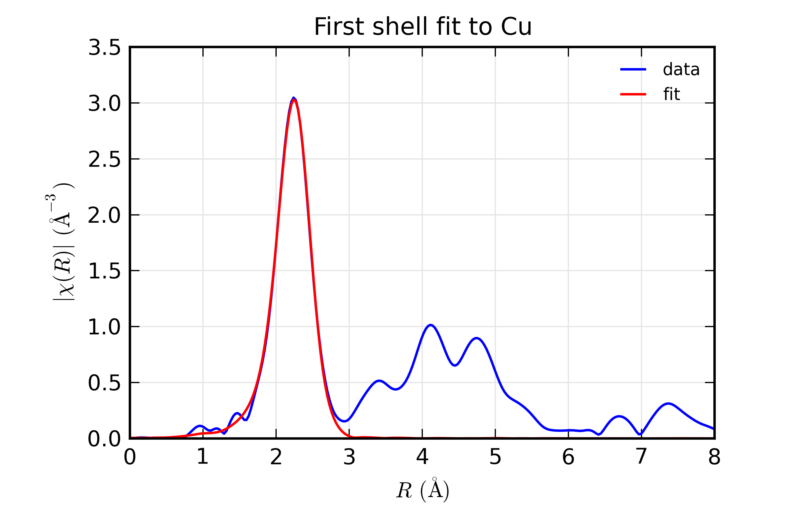
With plots of data and fits as shown below.

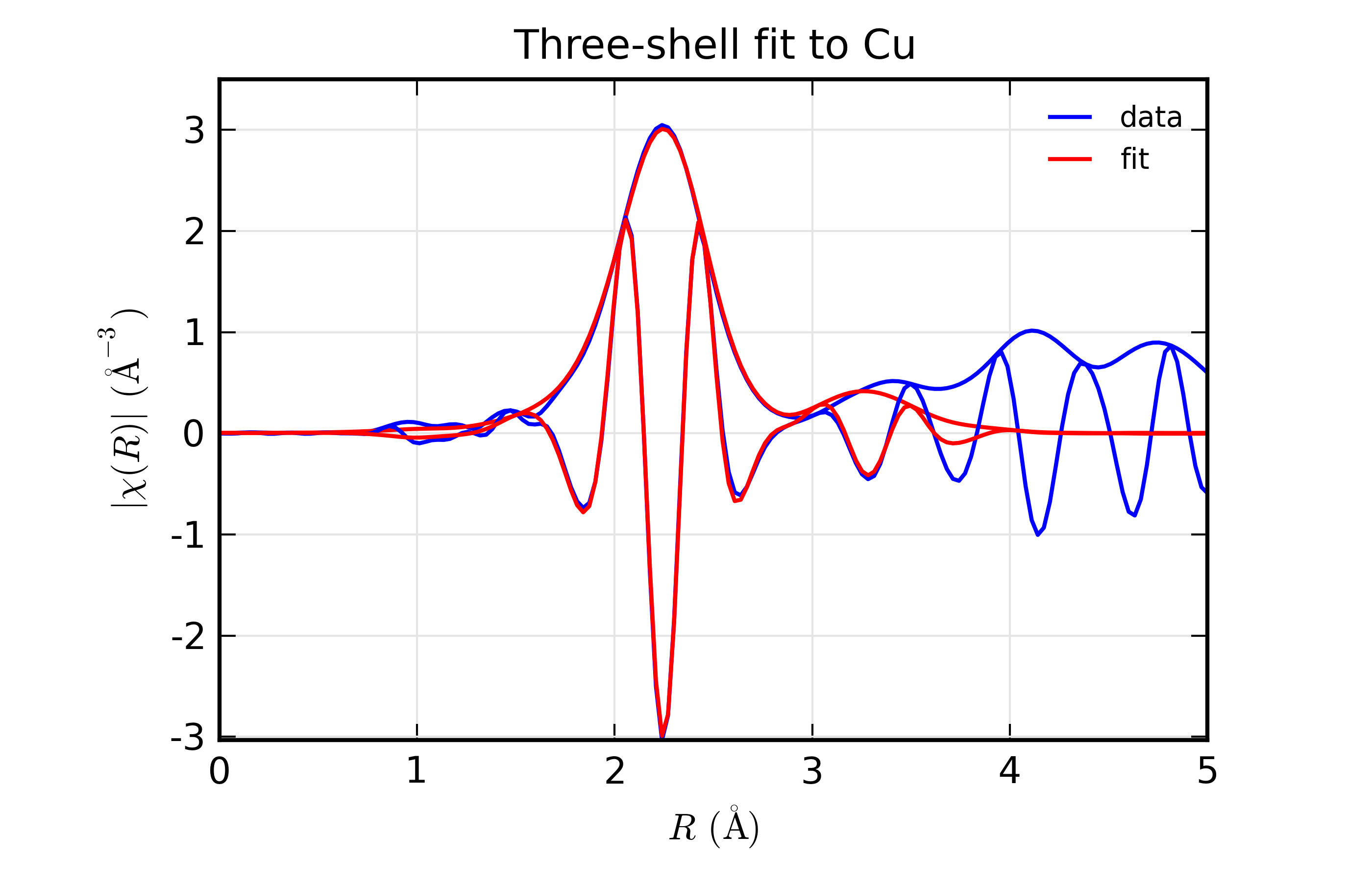
Figure 14.8.9.1 Results for Feffit for a 3-shell fit to a spectrum from Cu metal, constraining all path distances to expand with a single variable.
Here, we show both the magnitude and real part of \(\chi(R)\). The fit to the real part shows excellent agreement over the fit \(R\) range of [1.4, 3.4] \(\AA\). It is often useful the contributions from the individual paths. With the macros defined above, this is pretty straightforward, as we can just do:
plot_modelpaths_k(dset, offset=-1)
plot_modelpaths_r(dset, comp='re', offset=-1, xmax=6)
to generate the following plots of the contributions of the different paths:
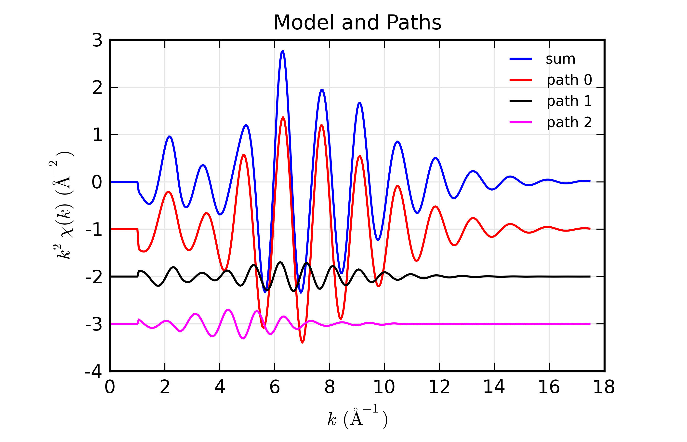
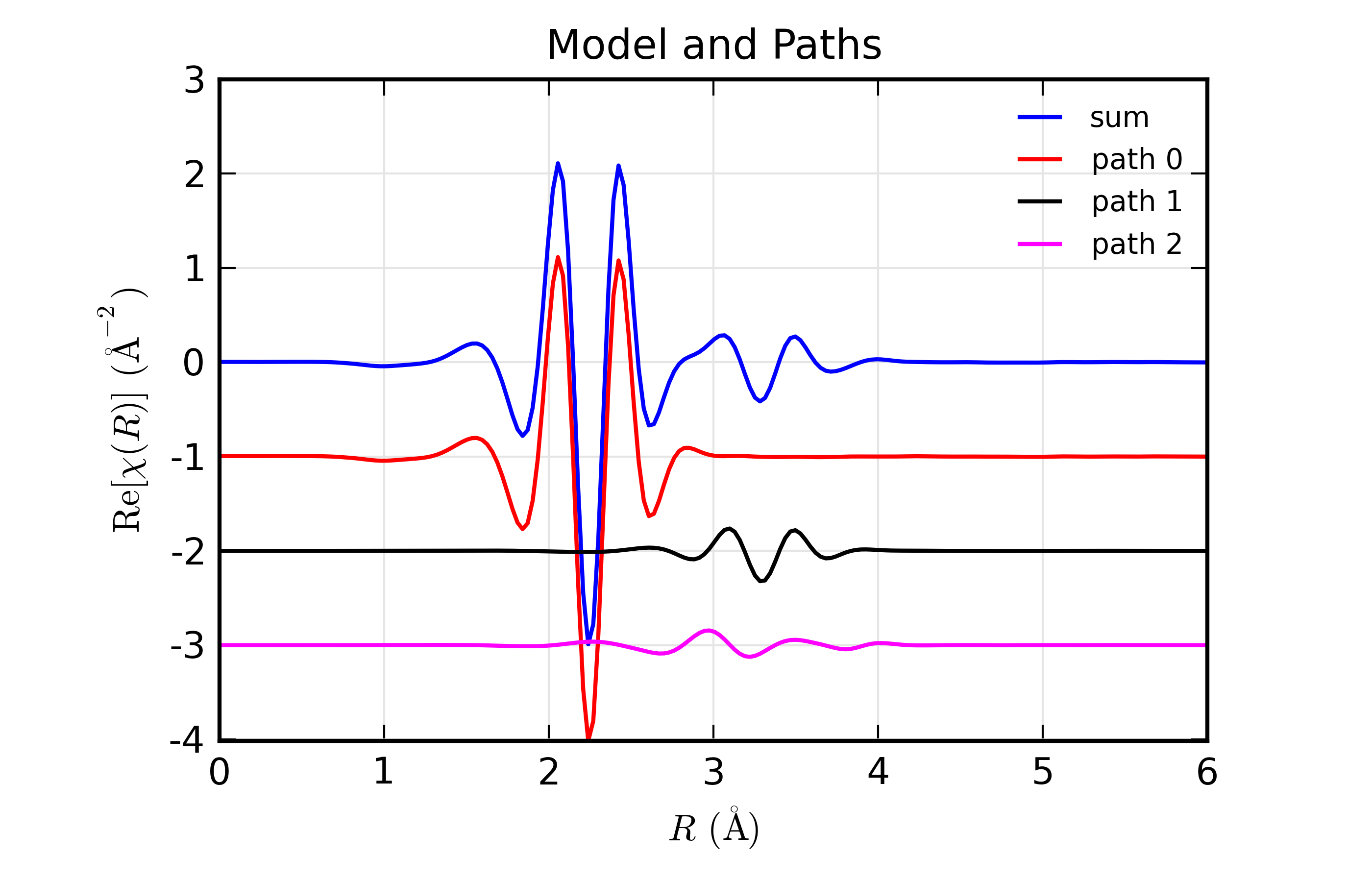
Figure 14.8.9.2 Path contributions to full mode for the 3-shell fit to Cu spectrum.
14.8.10. Example 3: Fit 3 datasets with 1 Path each
We’ll extend the above example by adding two more data sets. Since the three data sets have some things in common, we’ll be able to use some a smaller number of total variable parameters for all data sets than if we had fit each of them individually. This further allows us to reduce the number of freely varying parameters in a model of XAFS data, and to better measure the parameters that are varied.
Here, we’ll use data on Cu metal measured at three different temperatures. Since there is no phase change in the material over this temperature range, the structure changes in small and predictable ways that lends itself to simple parameterization. In the interest of brevity, we’ll only use one path, but the example could easily be extended to include more paths.
In this example, we have three distinct datasets, so we’ll have three lists
of paths. Each of these will have a single path. Since we’re modeling
nearly the same structure, the three paths will use the same Feff.dat file
and have many parameters in common, but some parameters will be different
for each data set. As with the previous example, we use the same amplitude
reduction factor \(E_0\) shift to all data sets. We allow distances to
vary, but constrain them so that the change is linear in the sample
temperature, as if there were a simple linear expansion in \(R\). To
do this, we set deltar = 'dr_off + T*alpha*reff', where T is the
temperature for the dataset. For \(\sigma^2\) we’ll use one of the
built-in models described in Models for Calculating sigma2. Here we’ll use sigma2_eins(), but
sigma2_debye() can be used as well, and does a better job for
multiple-scattering paths in simple systems. The model then uses 2
variable parameters for three temperature-dependent distances and 1
variable parameter for three temperature-dependent mean-square
displacements. The full script for the fit looks like this:
## examples/feffit/doc_feffit3.lar
# read 3 datasets
cu_10 = read_ascii('../xafsdata/cu_10k.xmu')
autobk(cu_10.energy, cu_10.mu, group=cu_10, rbkg=1.0, kw=2)
cu_50 = read_ascii('../xafsdata/cu_50k.xmu')
autobk(cu_50.energy, cu_50.mu, group=cu_50, rbkg=1.0, kw=2)
cu_150 = read_ascii('../xafsdata/cu_150k.xmu')
autobk(cu_150.energy, cu_150.mu, group=cu_150, rbkg=1.0, kw=2)
# define fitting parameter group
pars = group(amp = param(1, vary=True),
del_e0 = guess(2.0),
theta = param(250, min=10, vary=True),
dr_off = guess(0),
alpha = guess(0) )
# define 3 Feff Path, give expressions for Path Parameters
path1_10 = feffpath('feff0001.dat', s02 = 'amp', e0 = 'del_e0',
deltar = 'dr_off + 10*alpha*reff',
sigma2 = 'sigma2_eins(10, theta)')
path1_50 = feffpath('feff0001.dat', s02 = 'amp', e0 = 'del_e0',
deltar = 'dr_off + 50*alpha*reff',
sigma2 = 'sigma2_eins(50, theta)')
path1_150 = feffpath('feff0001.dat', s02 = 'amp', e0 = 'del_e0',
deltar = 'dr_off + 150*alpha*reff',
sigma2 = 'sigma2_eins(150, theta)')
trans = feffit_transform(kmin=3, kmax=17, kw=2, dk=4, window='kaiser', rmin=1.4, rmax=3.4)
# define 3 datasets, each with data, pathlist, transform for each
dset_10 = feffit_dataset(data=cu_10, pathlist=[path1_10], transform=trans)
dset_50 = feffit_dataset(data=cu_50, pathlist=[path1_50], transform=trans)
dset_150 = feffit_dataset(data=cu_150, pathlist=[path1_150], transform=trans)
# perform fit!
out = feffit(pars, [dset_10, dset_50, dset_150])
report = feffit_report(out)
print( report)
run('doc_macros.lar')
write_report('doc_feffit3.out', report)
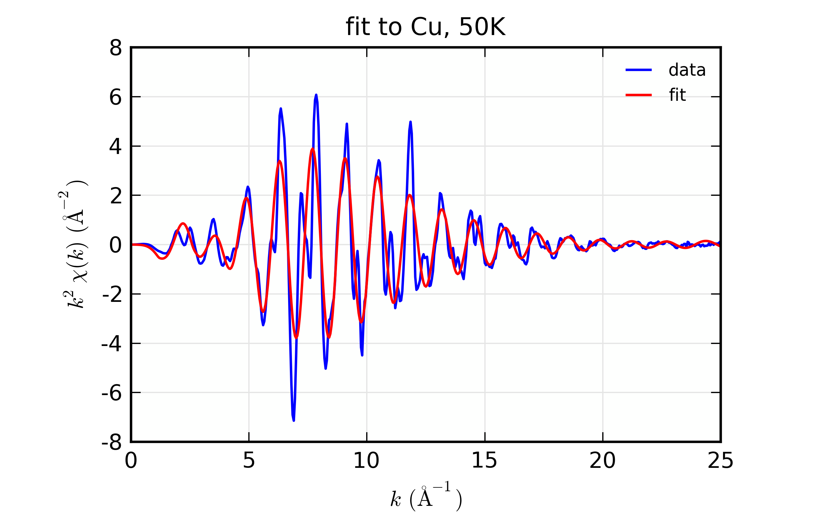
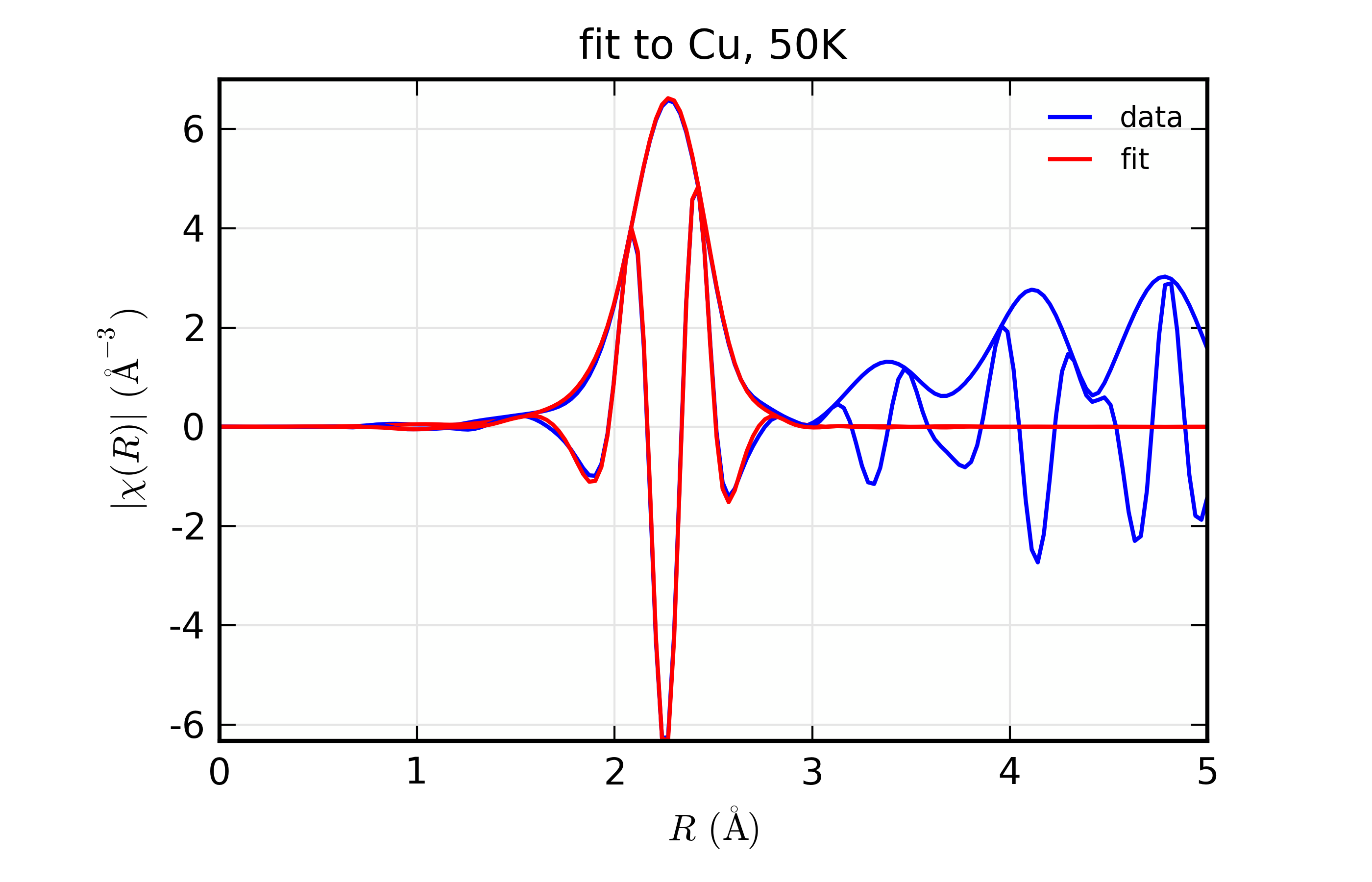
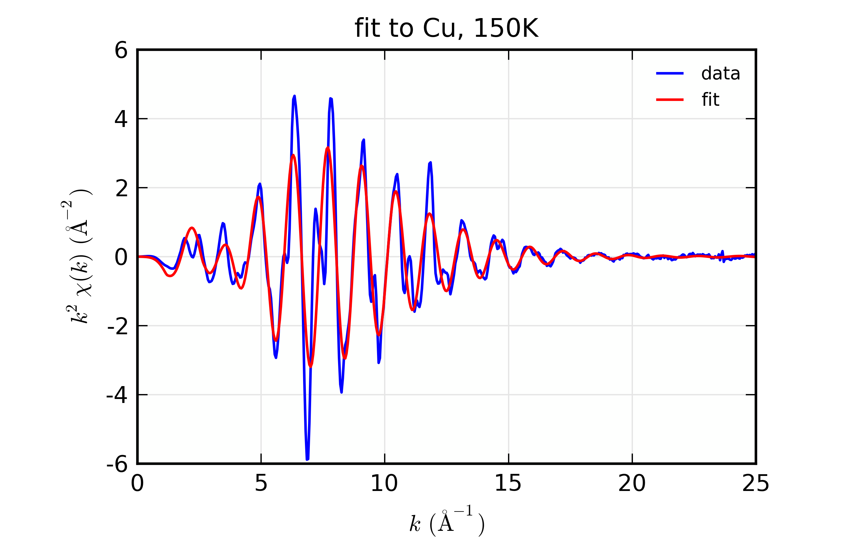
plot_chifit(dset_10, title='fit to Cu, 10K', rmax=5, win=1)
plot_chifit(dset_50, title='fit to Cu, 50K', rmax=5, win=3)
plot_chifit(dset_150, title='fit to Cu, 150K', rmax=5, win=5)
# ## end examples/feffit/doc_feffit3.lar
Here we read in 3 datasets for \(\mu(E)\) data and do the background subtraction on each of them. We define 5 fitting parameters, including the characteristic (here, Einstein) temperature which will determine the value of \(\sigma^2\), and two parameters for the linear temperature dependence of \(R\). The output for this fit is:
=================== FEFFIT RESULTS ====================
[[Statistics]]
  n_function_calls     = 25
  n_variables          = 5
  n_data_points        = 390
  n_independent        = 56.4760609
  chi_square           = 2965.82273
  reduced chi_square   = 57.6155727
  r-factor             = 0.01636032
  Akaike info crit     = 233.706924
  Bayesian info crit   = 243.876008

[[Variables]]
  alpha                =  5.2949e-6 +/- 6.6608e-6  (init= 0.0000000)
  amp                  =  0.8884690 +/- 0.0307237  (init= 1.0000000)
  del_e0               =  5.3732949 +/- 0.6134197  (init= 2.0000000)
  dr_off               = -3.0553e-4 +/- 0.0027193  (init= 0.0000000)
  theta                =  232.89303 +/- 8.0553391  (init= 250.00000)

[[Correlations]] (unreported correlations are <  0.100)
  amp, theta           = -0.854
  del_e0, dr_off       =  0.799
  alpha, dr_off        = -0.380
  alpha, del_e0        =  0.107

[[Dataset 1 of 3]]
  unique_id            = 'dzhvfzs6'
  fit space            = 'r'
  r-range              = 1.400, 3.400
  k-range              = 3.000, 17.000
  k window, dk         = 'kaiser', 4.000
  paths used in fit    = ['feff0001.dat']
  k-weight             = 2
  epsilon_k            = Array(mean=0.0011445, std=9.5328e-4)
  epsilon_r            = 0.0384678
  n_independent        = 18.825

[[Paths]]
 = Path 'p3tf6mewg' = Cu K Edge
    feffdat file = feff0001.dat, from feff run ''
    geometry  atom      x        y        z      ipot
              Cu       0.0000,  0.0000,  0.0000  0 (absorber)
              Cu       0.0000, -1.8016,  1.8016  1
     reff   =  2.5478000
     degen  =  12.000000
     n*s02  =  0.8884690 +/- 0.0307237  := 'amp'
     e0     =  5.3732949 +/- 0.6134197  := 'del_e0'
     r      =  2.5476294 +/- 0.0026594  := 'reff + dr_off + 10*alpha*reff'
     deltar = -1.7063e-4 +/- 0.0026594  := 'dr_off + 10*alpha*reff'
     sigma2 =  0.0032777 +/- 1.1337e-4  := 'sigma2_eins(10, theta)'

[[Dataset 2 of 3]]
  unique_id            = 'de4mv6pn'
  fit space            = 'r'
  r-range              = 1.400, 3.400
  k-range              = 3.000, 17.000
  k window, dk         = 'kaiser', 4.000
  paths used in fit    = ['feff0001.dat']
  k-weight             = 2
  epsilon_k            = Array(mean=0.0010793, std=0.0010405)
  epsilon_r            = 0.0362771
  n_independent        = 18.825

[[Paths]]
 = Path 'p3tf6mewg' = Cu K Edge
    feffdat file = feff0001.dat, from feff run ''
    geometry  atom      x        y        z      ipot
              Cu       0.0000,  0.0000,  0.0000  0 (absorber)
              Cu       0.0000, -1.8016,  1.8016  1
     reff   =  2.5478000
     degen  =  12.000000
     n*s02  =  0.8884690 +/- 0.0307237  := 'amp'
     e0     =  5.3732949 +/- 0.6134197  := 'del_e0'
     r      =  2.5481690 +/- 0.0025219  := 'reff + dr_off + 50*alpha*reff'
     deltar =  3.6899e-4 +/- 0.0025219  := 'dr_off + 50*alpha*reff'
     sigma2 =  0.0033405 +/- 1.2575e-4  := 'sigma2_eins(50, theta)'

[[Dataset 3 of 3]]
  unique_id            = 'durzhxyo'
  fit space            = 'r'
  r-range              = 1.400, 3.400
  k-range              = 3.000, 17.000
  k window, dk         = 'kaiser', 4.000
  paths used in fit    = ['feff0001.dat']
  k-weight             = 2
  epsilon_k            = Array(mean=7.3125e-4, std=0.0013139)
  epsilon_r            = 0.0245778
  n_independent        = 18.825

[[Paths]]
 = Path 'p3tf6mewg' = Cu K Edge
    feffdat file = feff0001.dat, from feff run ''
    geometry  atom      x        y        z      ipot
              Cu       0.0000,  0.0000,  0.0000  0 (absorber)
              Cu       0.0000, -1.8016,  1.8016  1
     reff   =  2.5478000
     degen  =  12.000000
     n*s02  =  0.8884690 +/- 0.0307237  := 'amp'
     e0     =  5.3732949 +/- 0.6134197  := 'del_e0'
     r      =  2.5495180 +/- 0.0029344  := 'reff + dr_off + 150*alpha*reff'
     deltar =  0.0017180 +/- 0.0029344  := 'dr_off + 150*alpha*reff'
     sigma2 =  0.0050382 +/- 2.9419e-4  := 'sigma2_eins(150, theta)'

=======================================================
Note that an uncertainty is estimated for the Path parameters, including
sigma2, which is calculated with the sigma2_eins() function.
Such derived uncertainties do reflect the uncertainties and correlations
between variables. For example, a simplistic evaluation for the standard
error in one of the sigma2 parameters using the estimated variance in
the theta might be done as follows:
larch> _ave = sigma2_eins(10, pars.theta)
larch> _dlo = sigma2_eins(10, pars.theta-pars.theta.stderr) - _ave
larch> _dhi = sigma2_eins(10, pars.theta+pars.theta.stderr) - _ave
larch> print "sigma2(T=10) = %.5f  (%+.5f, %+.5f)" % (_ave, _dlo, _dhi)
sigma2(T=10) = 0.00328  (+0.00011, -0.00011)
This gives an estimate about 3 times larger than the estimate automatically derived from the fit. The reason for this is that the simple evaluation ignores the correlation between parameters, which is taken into account in the automatically derived uncertainties. In this case, including this correlation significantly reduces the estimated uncertainty.
The output plots for the fits to the three datasets are given below.
 10 K, k-space
 10 K, R-space
 50 K, k-space
 50 K, R-space
 150 K, k-space
 150 K, R-space
Figure 14.8.10.1 Fit to Cu metal at 10 K, 50 K, and 150 K, from simultaneous fit to all 3 datasets with 5 variables used.
Again, in the interest of brevity and consistency through this chapter, these example are deliberately simple and meant to be illustrative of the capabilities and procedures and should not be viewed as limiting the types of problems that can be modeled.
14.8.11. Example 4: Measuring Coordination number
For this and the following example, we switch from Cu metal data to data on a simple metal oxide, FeO. The structure is a basic rock-salt structure, and we’ll model 2 paths for Fe-O and Fe-Fe in this structure. While the data is imperfect, we’ll use it to illustrate a few points in modeling EXAFS data.
For the examples above with Cu metal, we tacitly assumed that the
coordination number for the different paths was correct, and we adjusted an
\(S_0^2\) parameter. But, as with many analyses on real systems of
research interest, we’d like to fit the coordination number for the two
different paths here. To do this, we set an \(S_0^2\) parameter to a
fixed value, and also force degen (the number of equivalent paths in
the structure used to generate the Feff.dat files) to be 1 for each path.
Instead, we’ll define parameters n1 and n2, and set the Fe-O path’s
amplitude to be s02*n1 and the Fe-Fe path’s amplitude to be s02*n2.
We’ll allow n1 and n2 to vary in the fit, and also define variable
parameters for the other path parameters, including separate variables for
\(\Delta R\) and \(\sigma^2\). The script for this fit is below:
## examples/feffit/doc_feffit4.lar

feo_dat = read_ascii('../xafsdata/feo_xafs.dat', labels='energy mu')
autobk(feo_dat, kweight=2, rbkg=0.9)

# define fitting parameter group
pars = group(n1     = param(6, vary=True),
             n2     = param(12, vary=True),
             s02    = 0.700,
             de0    = guess(0.1),
             sig2_1 = param(0.002, vary=True),
             delr_1 = guess(0.),
             sig2_2 = param(0.002, vary=True),
             delr_2 = guess(0.)  )

# define Feff Paths, give expressions for Path Parameters
path_feo = feffpath('feff_feo01.dat',
                    degen = 1,
                    s02    = 's02*n1',
                    e0     = 'de0',
                    sigma2 = 'sig2_1',
                    deltar = 'delr_1')

path_fefe = feffpath('feff_feo02.dat',
                     degen = 1,
                     s02    = 's02*n2',
                     e0     = 'de0',
                     sigma2 = 'sig2_2',
                     deltar = 'delr_2')

# set tranform / fit ranges
trans = feffit_transform(kmin=2.0, kmax=13.5, kweight=3,
                         dk=3,  window='kaiser',
                         rmin=1.0, rmax=3.2, fitspace='r')

# define dataset to include data, pathlist, transform
dset  = feffit_dataset(data=feo_dat, pathlist=[path_feo, path_fefe],
                       transform=trans)
out = feffit(pars, dset)
print( feffit_report(out))
run('doc_macros.lar')
write_report('doc_feffit4.out', feffit_report(out))

plot_chifit(dset, title='Two-path fit to FeO')
## end examples/feffit/doc_feffit4.lar
The most important point here is the definitions used in setting up the
amplitudes for the paths: first, that we set degen to 1, and second
that we used the expression s02*n1 and so forth for the value of the
Path’s amplitude. A secondary note is that we gave two different
k-weights to feffit_transform(), which causes both k-weights to be
used in the fit.
The resulting output is
=================== FEFFIT RESULTS ====================
[[Statistics]]
  n_function_calls     = 65
  n_variables          = 7
  n_data_points        = 144
  n_independent        = 17.1064802
  chi_square           = 64.9851682
  reduced chi_square   = 6.43004950
  r-factor             = 0.01751179
  Akaike info crit     = 36.8320484
  Bayesian info crit   = 42.7082499

[[Variables]]
  de0                  = -1.4741655 +/- 1.1341834  (init= 0.1000000)
  delr_1               = -0.0293664 +/- 0.0107585  (init= 0.0000000)
  delr_2               =  0.0478234 +/- 0.0083873  (init= 0.0000000)
  n1                   =  5.5267534 +/- 1.2499525  (init= 6.0000000)
  n2                   =  11.407633 +/- 1.5333836  (init= 12.000000)
  sig2_1               =  0.0120204 +/- 0.0027069  (init= 0.0020000)
  sig2_2               =  0.0125357 +/- 0.0011737  (init= 0.0020000)

[[Correlations]] (unreported correlations are <  0.100)
  n2, sig2_2           =  0.939
  de0, delr_2          =  0.919
  n1, sig2_1           =  0.897
  de0, delr_1          =  0.582
  delr_1, delr_2       =  0.539
  delr_1, sig2_1       =  0.220
  delr_1, n1           =  0.190
  delr_2, sig2_2       =  0.184
  de0, n1              = -0.178
  delr_2, n2           =  0.159
  delr_2, n1           = -0.156
  de0, sig2_1          = -0.125
  delr_2, sig2_1       = -0.107
  n1, n2               =  0.106

[[Dataset]]
  unique_id            = 'da77uds7'
  fit space            = 'r'
  r-range              = 1.000, 3.200
  k-range              = 2.000, 13.500
  k window, dk         = 'kaiser', 3.000
  paths used in fit    = ['feff_feo01.dat', 'feff_feo02.dat']
  k-weight             = 3
  epsilon_k            = Array(mean=7.7074e-4, std=0.0018654)
  epsilon_r            = 0.1661149
  n_independent        = 17.106

[[Paths]]
 = Path 'pjuumtmhe' = Fe K Edge
    feffdat file = feff_feo01.dat, from feff run ''
    geometry  atom      x        y        z      ipot
              Fe       0.0000,  0.0000,  0.0000  0 (absorber)
               O       0.0000,  2.1387,  0.0000  1
     reff   =  2.1387000
     degen  =  1.0000000
     n*s02  =  3.8687274 +/- 0.8749668  := 's02*n1'
     e0     = -1.4741655 +/- 1.1341834  := 'de0'
     r      =  2.1093336 +/- 0.0107585  := 'reff + delr_1'
     deltar = -0.0293664 +/- 0.0107585  := 'delr_1'
     sigma2 =  0.0120204 +/- 0.0027069  := 'sig2_1'

 = Path 'p7etnrdqr' = Fe K Edge
    feffdat file = feff_feo02.dat, from feff run ''
    geometry  atom      x        y        z      ipot
              Fe       0.0000,  0.0000,  0.0000  0 (absorber)
              Fe       2.1387,  0.0000, -2.1387  2
     reff   =  3.0246000
     degen  =  1.0000000
     n*s02  =  7.9853429 +/- 1.0733686  := 's02*n2'
     e0     = -1.4741655 +/- 1.1341834  := 'de0'
     r      =  3.0724234 +/- 0.0083873  := 'reff + delr_2'
     deltar =  0.0478234 +/- 0.0083873  := 'delr_2'
     sigma2 =  0.0125357 +/- 0.0011737  := 'sig2_2'

=======================================================
with plots:
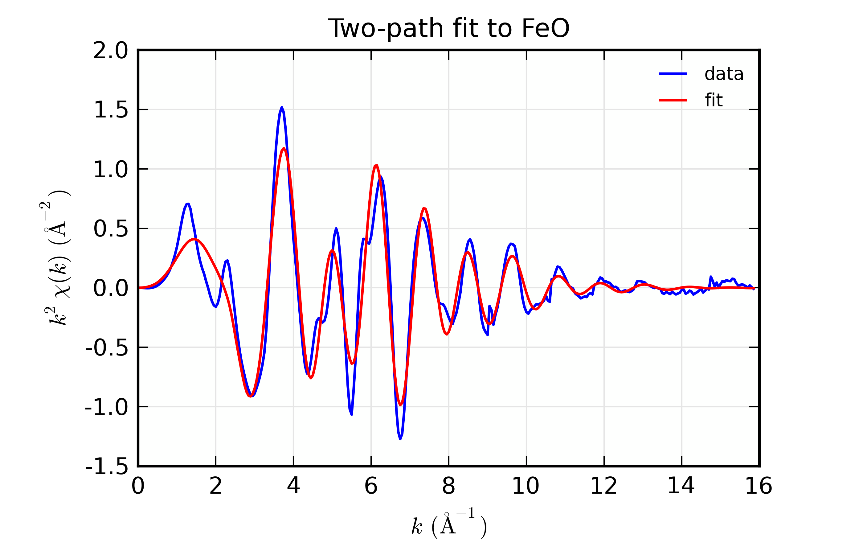 k-space
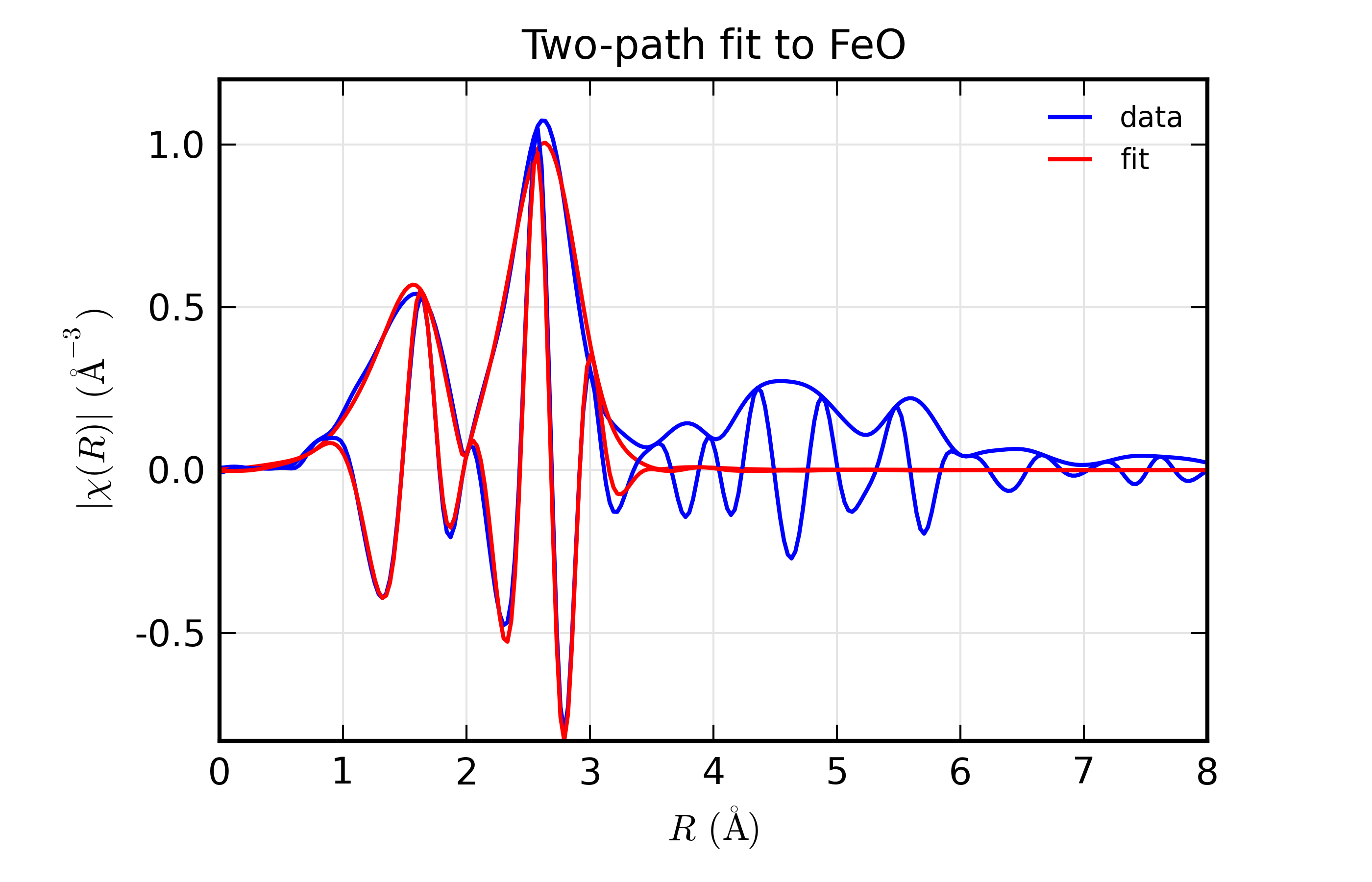 R-space
Figure 14.8.11.1 Fits to 2-path fit to FeO EXAFS
14.8.12. Example 5: Comparing Fits in different Fit Spaces
We now turn to comparing fits in unfiltered k-space, R-space, and filter k-space (or “q space”). This is partly to illustrate the preference for using R- or q-space for fitting, and partly to demonstrate how one can run similar fits and compare the results. We’ll use the FeO data from the previous example.
To change fitting models and transform parameters, we’ll make copies of the parameter groups and dataset groups, make a few changes, and re-run the fits. For example, we can change the fitting space with (see examples/feffit/doc_feffit5.lar):
larch> pars2 = copy(pars)   # copy parameters
larch> dset2 = copy(dset)   # copy dataset
larch> dset2.transform.fitspace = 'q'  # fit in backtransformed k-space
Now we can run feffit() with the new parameter group and Dataset
group, and compare the results either by plotting models from the different
copies of the dataset or by viewing the parameter values and fit statistics
with:
larch> out2  = feffit(pars2, dset2)
larch> print '*** R Space ***'
larch> print feffit_report(out, with_paths=False, min_correl=0.5)
larch> print '*** Q Space ***'
larch> print feffit_report(out2, with_paths=False, min_correl=0.5)
which gives
=================== FEFFIT RESULTS ====================
[[Statistics]]
  n_function_calls     = 65
  n_variables          = 7
  n_data_points        = 144
  n_independent        = 17.1064802
  chi_square           = 64.9851682
  reduced chi_square   = 6.43004950
  r-factor             = 0.01751179
  Akaike info crit     = 36.8320484
  Bayesian info crit   = 42.7082499

[[Variables]]
  de0                  = -1.4741655 +/- 1.1341834  (init= 0.1000000)
  delr_1               = -0.0293664 +/- 0.0107585  (init= 0.0000000)
  delr_2               =  0.0478234 +/- 0.0083873  (init= 0.0000000)
  n1                   =  5.5267534 +/- 1.2499525  (init= 6.0000000)
  n2                   =  11.407633 +/- 1.5333836  (init= 12.000000)
  sig2_1               =  0.0120204 +/- 0.0027069  (init= 0.0020000)
  sig2_2               =  0.0125357 +/- 0.0011737  (init= 0.0020000)

[[Correlations]] (unreported correlations are <  0.500)
  n2, sig2_2           =  0.939
  de0, delr_2          =  0.919
  n1, sig2_1           =  0.897
  de0, delr_1          =  0.582
  delr_1, delr_2       =  0.539

[[Dataset]]
  unique_id            = 'da77uds7'
  fit space            = 'r'
  r-range              = 1.000, 3.200
  k-range              = 2.000, 13.500
  k window, dk         = 'kaiser', 3.000
  paths used in fit    = ['feff_feo01.dat', 'feff_feo02.dat']
  k-weight             = 3
  epsilon_k            = Array(mean=7.7074e-4, std=0.0018654)
  epsilon_r            = 0.1661149
  n_independent        = 17.106
=======================================================
=================== FEFFIT RESULTS ====================
[[Statistics]]
  n_function_calls     = 65
  n_variables          = 7
  n_data_points        = 230
  n_independent        = 17.1064802
  chi_square           = 156.348404
  reduced chi_square   = 15.4701142
  r-factor             = 0.01377419
  Akaike info crit     = 51.8503032
  Bayesian info crit   = 57.7265047

[[Variables]]
  de0                  = -1.4418399 +/- 1.0075979  (init= 0.1000000)
  delr_1               = -0.0291715 +/- 0.0095887  (init= 0.0000000)
  delr_2               =  0.0481107 +/- 0.0074656  (init= 0.0000000)
  n1                   =  5.6991167 +/- 1.1559886  (init= 6.0000000)
  n2                   =  11.460975 +/- 1.3706924  (init= 12.000000)
  sig2_1               =  0.0123871 +/- 0.0024544  (init= 0.0020000)
  sig2_2               =  0.0125804 +/- 0.0010458  (init= 0.0020000)

[[Correlations]] (unreported correlations are <  0.500)
  n2, sig2_2           =  0.940
  de0, delr_2          =  0.919
  n1, sig2_1           =  0.900
  de0, delr_1          =  0.585
  delr_1, delr_2       =  0.542

[[Dataset]]
  unique_id            = 'da77uds7'
  fit space            = 'q'
  r-range              = 1.000, 3.200
  k-range              = 2.000, 13.500
  k window, dk         = 'kaiser', 3.000
  paths used in fit    = ['feff_feo01.dat', 'feff_feo02.dat']
  k-weight             = 3
  epsilon_k            = Array(mean=7.7074e-4, std=0.0018654)
  epsilon_r            = 0.1661149
  n_independent        = 17.106
=======================================================
We can see that the results are not very different – the best fit values and uncertainties for the varied parameters are quite close for the fit in ‘R’ space and ‘Q’ space.
Now, we can try the fit in unfiltered ‘K’ space:
larch> pars3 = copy(pars)   # copy parameters
larch> dset3 = copy(dset)   # copy dataset
larch> dset3.transform.kweight = 2
larch> dset3.transform.fitspace = 'k'
larch> out3 = feffit(pars3, dset3)
larch  print feffit_report(out3, with_paths=False, min_correl=0.5)
(we need to specify only one k-weight for a k-space fit) which gives:
=================== FEFFIT RESULTS ====================
[[Statistics]]
  n_function_calls     = 49
  n_variables          = 7
  n_data_points        = 230
  n_independent        = 17.1064802
  chi_square           = 7472994.14
  reduced chi_square   = 739425.988
  r-factor             = 0.14252657
  Akaike info crit     = 236.167828
  Bayesian info crit   = 242.044030

[[Variables]]
  de0                  = -1.8796930 +/- 2.5288417  (init= 0.1000000)
  delr_1               = -0.0289651 +/- 0.0316889  (init= 0.0000000)
  delr_2               =  0.0447213 +/- 0.0247359  (init= 0.0000000)
  n1                   =  5.0911303 +/- 2.4586464  (init= 6.0000000)
  n2                   =  12.781266 +/- 5.1119625  (init= 12.000000)
  sig2_1               =  0.0104533 +/- 0.0077437  (init= 0.0020000)
  sig2_2               =  0.0135407 +/- 0.0042583  (init= 0.0020000)

[[Correlations]] (unreported correlations are <  0.500)
  n2, sig2_2           =  0.924
  n1, sig2_1           =  0.881
  de0, delr_2          =  0.870
  de0, delr_1          =  0.671
  delr_1, delr_2       =  0.591

[[Dataset]]
  unique_id            = 'da77uds7'
  fit space            = 'k'
  r-range              = 1.000, 3.200
  k-range              = 2.000, 13.500
  k window, dk         = 'kaiser', 3.000
  paths used in fit    = ['feff_feo01.dat', 'feff_feo02.dat']
  k-weight             = 2
  epsilon_k            = Array(mean=8.0580e-4, std=0.0018556)
  epsilon_r            = 0.0152209
  n_independent        = 17.106
=======================================================
This has pretty similar best-fit values, but dramatically larger estimates of the errors. The spectrum is really very poorly fit in k-space because we have not accounted for the higher R components. Using R (and Q) space, we’re able to limit the R range used in determining the parameter values, estimated uncertainties, and the goodness-of-fit statistics. But since we can’t place these limits on what portion of the data is being compared to the model spectra in unfiltered k-space fit, the uncertainties reflect the fact that the full experimental spectrum is not well model. This is why it is recommended to not fit in unfiltered k space: the uncertainties in the parameters is too large.
Finally, we can also fit simultaneously in ‘k’ and ‘r’ space by making use of wavelet transforms (see Section XAFS: Wavelet Transforms for XAFS). For this, we specify both k and R ranges, and the fit is done on the wavelet transform. This gives:
=================== FEFFIT RESULTS ====================
[[Statistics]]
  n_function_calls     = 57
  n_variables          = 7
  n_data_points        = 33120
  n_independent        = 17.1064802
  chi_square           = 821.617284
  reduced chi_square   = 81.2960857
  r-factor             = 0.00997058
  Akaike info crit     = 80.2331669
  Bayesian info crit   = 86.1093683

[[Variables]]
  de0                  = -1.9314719 +/- 0.8311485  (init= 0.1000000)
  delr_1               = -0.0304702 +/- 0.0088736  (init= 0.0000000)
  delr_2               =  0.0444351 +/- 0.0069502  (init= 0.0000000)
  n1                   =  6.0513190 +/- 1.2911656  (init= 6.0000000)
  n2                   =  12.171926 +/- 1.2495291  (init= 12.000000)
  sig2_1               =  0.0131212 +/- 0.0029093  (init= 0.0020000)
  sig2_2               =  0.0131444 +/- 0.0010217  (init= 0.0020000)

[[Correlations]] (unreported correlations are <  0.500)
  n2, sig2_2           =  0.944
  de0, delr_2          =  0.928
  n1, sig2_1           =  0.917
  de0, delr_1          =  0.519

[[Dataset]]
  unique_id            = 'da77uds7'
  fit space            = 'w'
  r-range              = 1.000, 3.200
  k-range              = 2.000, 13.500
  k window, dk         = 'kaiser', 3.000
  paths used in fit    = ['feff_feo01.dat', 'feff_feo02.dat']
  k-weight             = 2
  epsilon_k            = Array(mean=8.0580e-4, std=0.0018556)
  epsilon_r            = 0.0152209
  n_independent        = 17.106
=======================================================
As you can see, the results are all pretty similar.
Of course, for all these examples, we’ve changed only one thing between these fits – the fitting ‘space’. The process of copying the parameter group and dataset, making modifications and re-doing fits can also include changing what parametres are varied, and what constraints are placed between parameters.
14.8.13. Example 6: Testing EXAFS sensitivity to \(Z\)
EXAFS is known to be sensitive to the atomic number \(Z\) of the scattering atom. This is due to the \(Z\) dependence of the scattering amplitude and phase shift (\(f(k)\) and \(\delta(k)\) in the EXAFS Equation of Section The EXAFS Equation using Feff and FeffPath Groups). A rule-of-thumb that is often stated is that EXAFS is sensitive to \(Z \pm 5\), or perhaps pessimistically to row of the Periodic Table, but not as sensitive as \(Z \pm 1\). Occassionally, you may see work that claims very fine \(Z\) sensitivity, such as being able to distinguish N and O ligands. In those works, XAFS results are typically used with chemical arguments about steric effects or known bond distances.
In this section, we’ll explore the \(Z\) sensitivity of XAFS with real data, by constructing Feff paths with different scatterers and trying to fit data with these different scattering paths. This makes a nice exercise in how to manipulate Feff, how to fit XAFS data, and how to compare XAFS fits. Just to make it a little more complicated, we’ll also explore the idea of Phase corrected Fourier transforms and how they might be used to better determine both \(R\) and \(Z\). The example script here is a little more complex than what we’ve seen above, using many feature of the Larch scripting language to do repeated fits and mathematically manipulating the arrays of data.
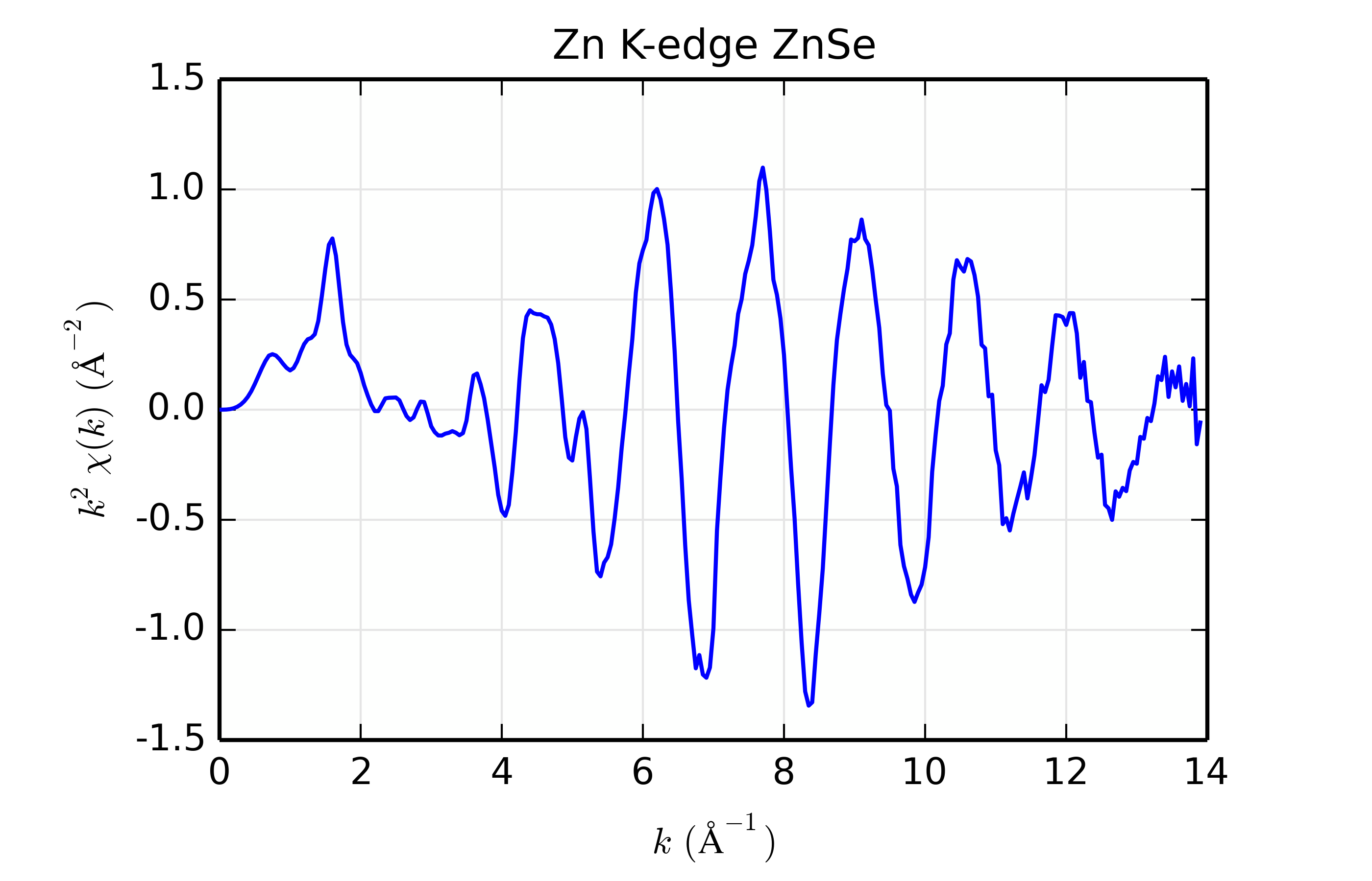
Figure 14.8.13.1 Zn K-edge XAFS data for ZnSe.
For this example, we’ll use Zn K-edge data of ZnSe, with \(\chi(k)\) data shown in Figure 14.8.13.1. The data is pretty good but not perfect, and is useful for the study here mainly because the structure is simple, with a well-isolated and well-ordered shell of scatterers (the cubic ZnS structure with 1 Zn site surrounded by 4 Se at 2.45 \(\rm\AA\)). While we’re sure that the scatterer should be Se, we’ll try scatterers of Zn, Ge, Se, Br, and Rb, spanning a small but sufficient range of \(Z\).
To construct the scattering paths, we’ll modify a Feff input file. To do
this, we start with a feff.inp file generated for crystalline ZnSe by the
ATOMS program, and add an IPOT to the list of atomic potentials (here the
line 3 35 Br), and then replace the IPOTs for 1 of the neighboring Se
atoms (that is, replacing a 2 with a 3, and changing the tag for
convenience). The resulting feff.inp file for Br looks this:
 TITLE  ZnSe (cubic zinc sulfide structure)
 HOLE 1   1.0   *  Zn K edge  (9659.0 eV), second number is S0^2

 CONTROL   1      1     1     1
 PRINT     1      0     0     0
 RMAX      6.0
 NLEG      4

 POTENTIALS
 *    ipot   Z  element
        0   30   Zn
        1   30   Zn
        2   34   Se
        3   36   Kr
      # 3   33   As
      # 3   32   Ge
      # 3   31   Ga

 ATOMS                          * this list contains 35 atoms
 *   x          y          z      ipot  tag              distance
    0.00000    0.00000    0.00000  0 Zn1             0.00000
    1.41690    1.41690    1.41690  2 Se1_1           2.45414
   -1.41690   -1.41690    1.41690  3 Br_1            2.45414
   -1.41690    1.41690   -1.41690  2 Se1_1           2.45414
    1.41690   -1.41690   -1.41690  2 Se1_1           2.45414
    2.83380    2.83380    0.00000  1 Zn1_1           4.00760
   -2.83380    2.83380    0.00000  1 Zn1_1           4.00760
    2.83380   -2.83380    0.00000  1 Zn1_1           4.00760
   -2.83380   -2.83380    0.00000  1 Zn1_1           4.00760
    2.83380    0.00000    2.83380  1 Zn1_1           4.00760
   -2.83380    0.00000    2.83380  1 Zn1_1           4.00760
    0.00000    2.83380    2.83380  1 Zn1_1           4.00760
    0.00000   -2.83380    2.83380  1 Zn1_1           4.00760
    2.83380    0.00000   -2.83380  1 Zn1_1           4.00760
   -2.83380    0.00000   -2.83380  1 Zn1_1           4.00760
    0.00000    2.83380   -2.83380  1 Zn1_1           4.00760
    0.00000   -2.83380   -2.83380  1 Zn1_1           4.00760
   -4.25070    1.41690    1.41690  2 Se1_2           4.69933
   -1.41690    4.25070    1.41690  2 Se1_2           4.69933
    4.25070   -1.41690    1.41690  2 Se1_2           4.69933
    1.41690   -4.25070    1.41690  2 Se1_2           4.69933
   -1.41690    1.41690    4.25070  2 Se1_2           4.69933
    1.41690   -1.41690    4.25070  2 Se1_2           4.69933
    4.25070    1.41690   -1.41690  2 Se1_2           4.69933
    1.41690    4.25070   -1.41690  2 Se1_2           4.69933
   -4.25070   -1.41690   -1.41690  2 Se1_2           4.69933
   -1.41690   -4.25070   -1.41690  2 Se1_2           4.69933
    1.41690    1.41690   -4.25070  2 Se1_2           4.69933
   -1.41690   -1.41690   -4.25070  2 Se1_2           4.69933
    5.66760    0.00000    0.00000  1 Zn1_2           5.66760
   -5.66760    0.00000    0.00000  1 Zn1_2           5.66760
    0.00000    5.66760    0.00000  1 Zn1_2           5.66760
    0.00000   -5.66760    0.00000  1 Zn1_2           5.66760
    0.00000    0.00000    5.66760  1 Zn1_2           5.66760
    0.00000    0.00000   -5.66760  1 Zn1_2           5.66760
 END
Afer running feff.inp, we collect the resulting feffNNNN.dat files –
either feff0001.dat or feff0002.dat will have the replaced scatterer,
the other will have Se as the scatterer. Once we’ve collected all these
files for runs of Feff with feff.inp altered for each scatterer, we’re ready
to do the fits.
The script to compare the fits will loop over these different scattering paths, doing a fit for each path, and store the results. This takes advantage of several features of the Larch scripting capabilities, including defining functions, and constructs like loops and dictionaries, as well as mathematical manipulation of the resulting arrays for the phase correction. The full script is:
## examples/feffit/doc_feffit6.lar

# Testing sensitivity to Z of backscatterer, and
# how well "phase corrected" Fourier transforms predict distance

def get_zinc_mu(filename, labels='energy dwelltime i0 i1'):
    """read raw data, do background subtraction"""
    dat = read_ascii(filename, labels=labels)
    dat.mu = -ln(dat.i1 / dat.i0)
    autobk(dat, e0 = 9666.0, rbkg=1.25, kweight=2)
    return dat
#enddef

def plot_chidata(data, title, win=1):
    kopts = dict(xlabel=r'$k \rm\,(\AA^{-1})$',
                 ylabel=r'$k^2\chi(k) \rm\,(\AA^{-2})$',
                 title=title, xmax=14, new=True, win=win)
    plot(data.k, data.chi*data.k**2, title=title, **kopts)
#enddef

def rplot_fit(dset, title, win=1):
    "make R-spae plots of results"
    ropts = dict(xlabel=r'$R \rm\,(\AA)$',
                 ylabel=r'$|\chi(R)| \rm\,(\AA^{-3})$',
                 title=title, xmax=6, win=win, show_legend=True)
    plot(dset.data.r,  dset.data.chir_mag, new=True, label='data', **ropts)
    plot(dset.model.r,  dset.model.chir_mag,  label='Feff Path', win=win)

    chir_pha = dset.model.chir_phcor
    chir_pha_mag = sqrt(chir_pha.real**2 + chir_pha.imag**2)
    plot(dset.model.r,  chir_pha_mag,  win=win, label='phase-corrected data')

    # find region around peak in phase-corrected chi(R)

    irmax = where(chir_pha_mag == max(chir_pha_mag))[0][0]
    x = dset.model.r[irmax-1: irmax+2]
    y = dset.model.chir_im[irmax-1: irmax+2]
    plot(x, y, win=win, color='black', style='short dashed',
         marker='o', label='Im[phase-corrected]')
    return
#enddef

def phase_correct(dset):
   "calculate phase-corrected FT, find estimate of R"
   nrpts = len(dset.model.r)
   path1 = list(dset.paths.items())[0][1]
   # get phase from Feff path
   feff_pha = interp(path1._feffdat.k, path1._feffdat.pha, dset.model.k)
   # phase-corrected Fourier Transform
   chir_pha = xftf_fast(dset.data.chi * exp(0-1j*feff_pha) *
                        dset.data.kwin * dset.data.k**2)[:nrpts]
   chir_pha_mag = sqrt(chir_pha.real**2 + chir_pha.imag**2)
   dset.model.chir_phcor = chir_pha

   # find region around peak in phase-corrected chi(R)
   irmax = where(chir_pha_mag == max(chir_pha_mag))[0][0]
   x = dset.model.r[irmax-1: irmax+2]
   y = dset.model.chir_im[irmax-1: irmax+2]
   # find where Im[chi(R)_phase_corrected] = 0: use linear regression
   o = linregress(y, x)
   dset.model.rphcor = o[1]
   return o[1]
#enddef

###################################################
znse_data = get_zinc_mu('../xafsdata/znse_zn_xafs.001',
                        labels='energy dwelltime i0 i1')

# plot_chidata(znse_data, 'Zn K-edge ZnSe')

# define Feff Paths, storing them in dictionary
paths = {}
pathargs = dict(degen=4.0, s02='amp', e0='del_e0', sigma2='sig2', deltar='del_r')
paths['Zn'] = feffpath('Feff_ZnSe/feff_znzn.dat', **pathargs)
paths['Ga'] = feffpath('Feff_ZnSe/feff_znga.dat', **pathargs)
paths['Ge'] = feffpath('Feff_ZnSe/feff_znge.dat', **pathargs)
paths['As'] = feffpath('Feff_ZnSe/feff_znas.dat', **pathargs)
paths['Se'] = feffpath('Feff_ZnSe/feff_znse.dat', **pathargs)
paths['Br'] = feffpath('Feff_ZnSe/feff_znbr.dat', **pathargs)
paths['Kr'] = feffpath('Feff_ZnSe/feff_znkr.dat', **pathargs)
paths['Rb'] = feffpath('Feff_ZnSe/feff_znrb.dat', **pathargs)

# set FT tranform and Fit ranges
trans = feffit_transform(rmin=1.5, rmax=3.0, kmin=3, kmax=13,
                         kw=2, dk=4, window='kaiser')

# perform fit for each scatterer
print( '|Scatterer|RedChi2|    S02     |   sigma2      |      E0     |      R       |R_phcor|')
fmt = '|  %s     | %5.1f |%s|%s|%s|%s|%7.3f|'

results = {}
for ix, scatterer in enumerate(('Zn', 'Ga', 'Ge', 'As', 'Se', 'Br', 'Kr', 'Rb')):
    dset  = feffit_dataset(data=znse_data, paths={scatterer: paths[scatterer]},
                           transform=trans)
    pars = group(amp    = guess(1.0),
                 del_e0 = guess(0.1, min=-20, max=20),
                 sig2   = param(0.006, vary=True, min=0),
                 del_r  = guess(0.) )

    out = feffit(pars, dset)
    path1 = out.datasets[0].paths[scatterer]
    # read scatterer from Feff geometry, to be sure it's correct
    scatt = path1._feffdat.geom[1][0]
    title = 'Path: Zn-%s ' % scatt
    r_phcor = phase_correct(out.datasets[0])
    rplot_fit(out.datasets[0], title, win=1+ix)

    redchi = out.chi2_reduced

    _amp   = '%5.2f(%.2f) ' % (out.params['amp'].value, out.params['amp'].stderr)
    _de0   = '%6.2f(%.2f) ' % (out.params['del_e0'].value,  out.params['del_e0'].stderr)
    _ss2   = '%6.4f(%.4f) ' % (out.params['sig2'].value,  out.params['sig2'].stderr)
    _r     = '%6.3f(%.3f) ' % (path1.reff+out.params['del_r'].value, out.params['del_r'].stderr)
    print( fmt % (scatt, redchi, _amp, _ss2, _de0, _r, r_phcor))
    results[scatterer] = out
#endfor

## end examples/feffit/doc_feffit6.lar
After reading in the data, the script builds Feff Paths, putting them into a dictionary. After define the fitting transform range, the script loops over each of the scatterers, doing a simple first-shell fit with each. The the phase-corrected \(\chi(R)\) is then calculated, and the peak value of \(R\) is found for this array. Finally, results are printed out.
Table of ZnSe Results. The results from fitting ZnSe XAFS data to scattering paths of Zn-Zn, Zn-Ge, Zn-Se, Zn-Br, and Zn-Rb. All paths started at the nominal distance of 2.454 \(\rm\AA\).
Scatterer
reduced chi-square
\(S_0^2\)
\(\sigma^2\)
\(E_0\)
\(R\)
\(R_{\rm{ph cor}}\)
Zn (30)
57.5
0.73(0.07)
0.0040(0.0006)
-7.98(1.23)
2.471(0.006)
2.451
Ge (32)
32.4
0.90(0.06)
0.0050(0.0005)
-2.99(0.93)
2.461(0.004)
2.457
Se (34)
12.7
0.89(0.04)
0.0059(0.0003)
0.09(0.58)
2.448(0.003)
2.461
Br (35)
16.7
1.08(0.06)
0.0070(0.0004)
1.71(0.79)
2.444(0.003)
2.462
Rb (37)
88.7
1.10(0.14)
0.0073(0.0009)
5.27(1.42)
2.425(0.007)
2.467
The results of the fits are given in the Table of ZnSe Results, with graphs below showing fits to the 5 different scatterers. The dependence of the results on \(Z\) of the back-scattering atom is seen to be reasonably strong. The values for reduced chi-square definitely indicate that Zn-Se is the best fit, and the values for the fitted parameters have rather clear correlations with \(Z\) – \(S_0^2\), \(\sigma^2\), and \(E_0\) increase with \(Z\), while \(R\) decreases. If anything, the \(Z \pm 5\) rule-of-thumb seems pessimistic, though the fits with Ge and Br look decent enough that it would be easy to conclude that \(Z \pm 2\) is reasonable.
As a curious side note, we note that \(S_0^2\) increases with
\(Z\). The scattering factor should also increase with \(Z\), which
might lead us to suspect a trend in the opposite direction. The confounding
factor here is \(\sigma^2\) – if we fix \(\sigma^2\) to 0.006 (by
changing vary=True to vary=False) and re-run the fits, \(S_0^2\)
has a slight negative dependence on \(Z\).
 Zn
Zn
 Ge
Ge
 Se
Se
 Br
Br
 Rb
Rb
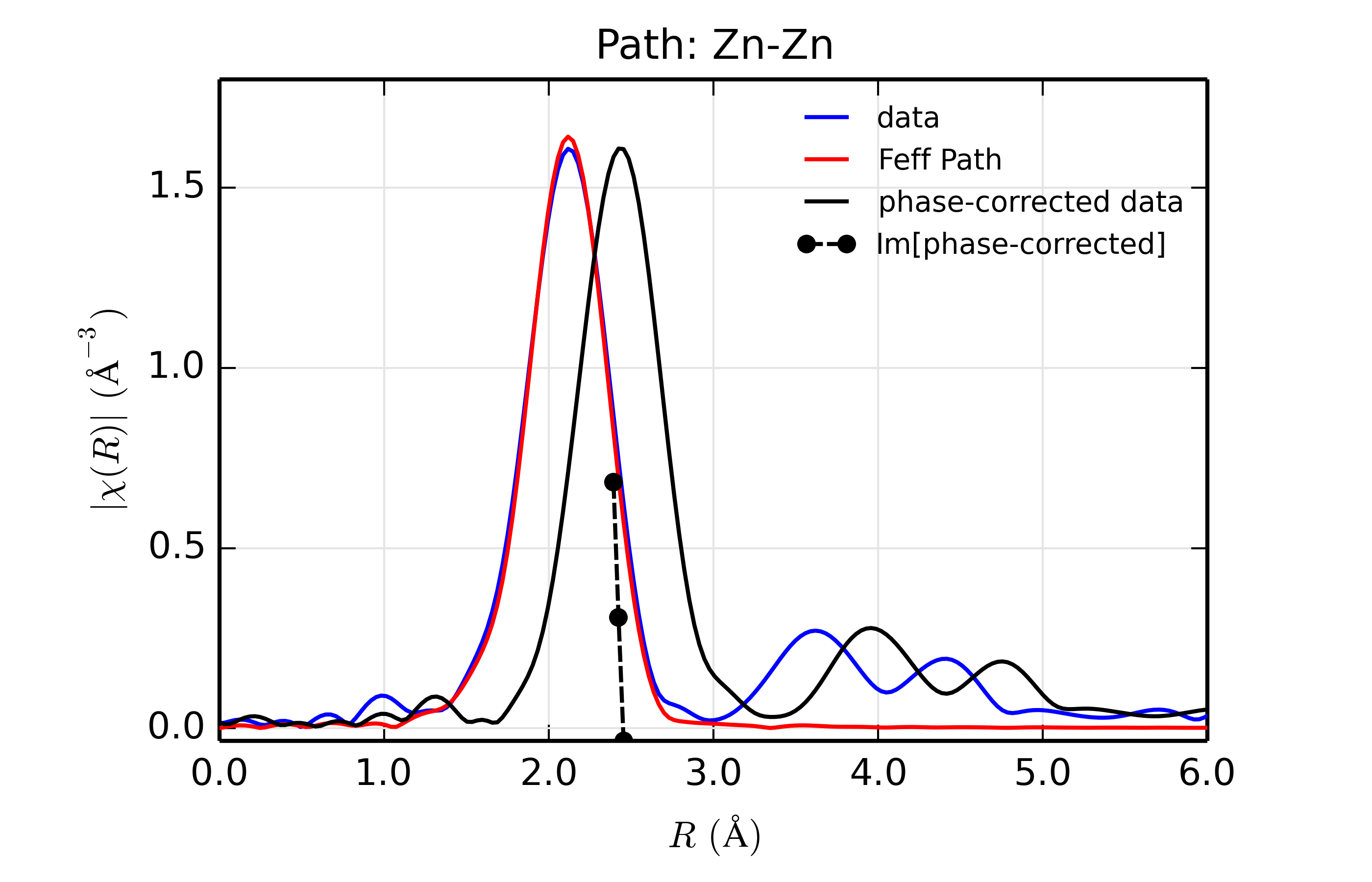
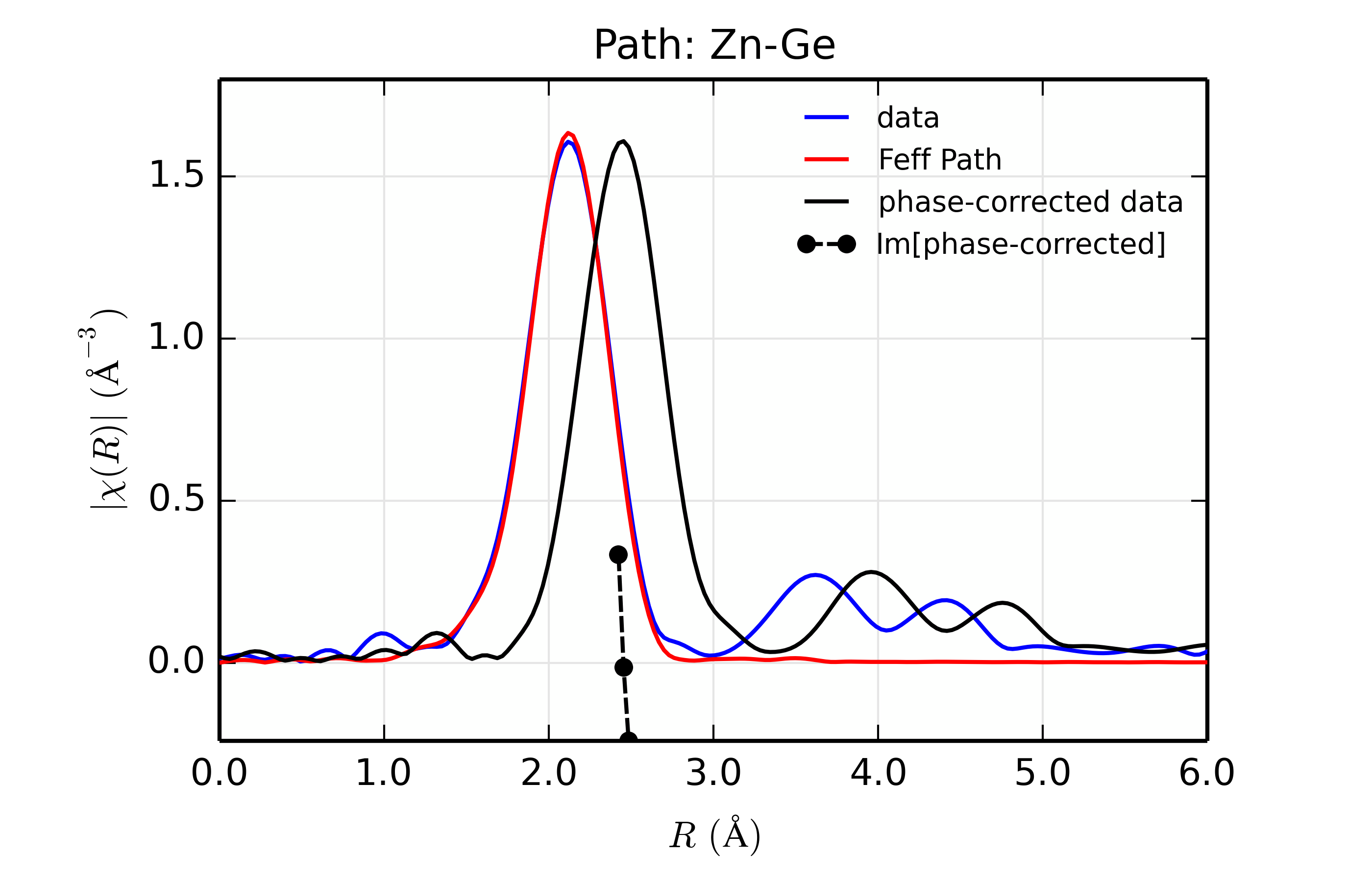
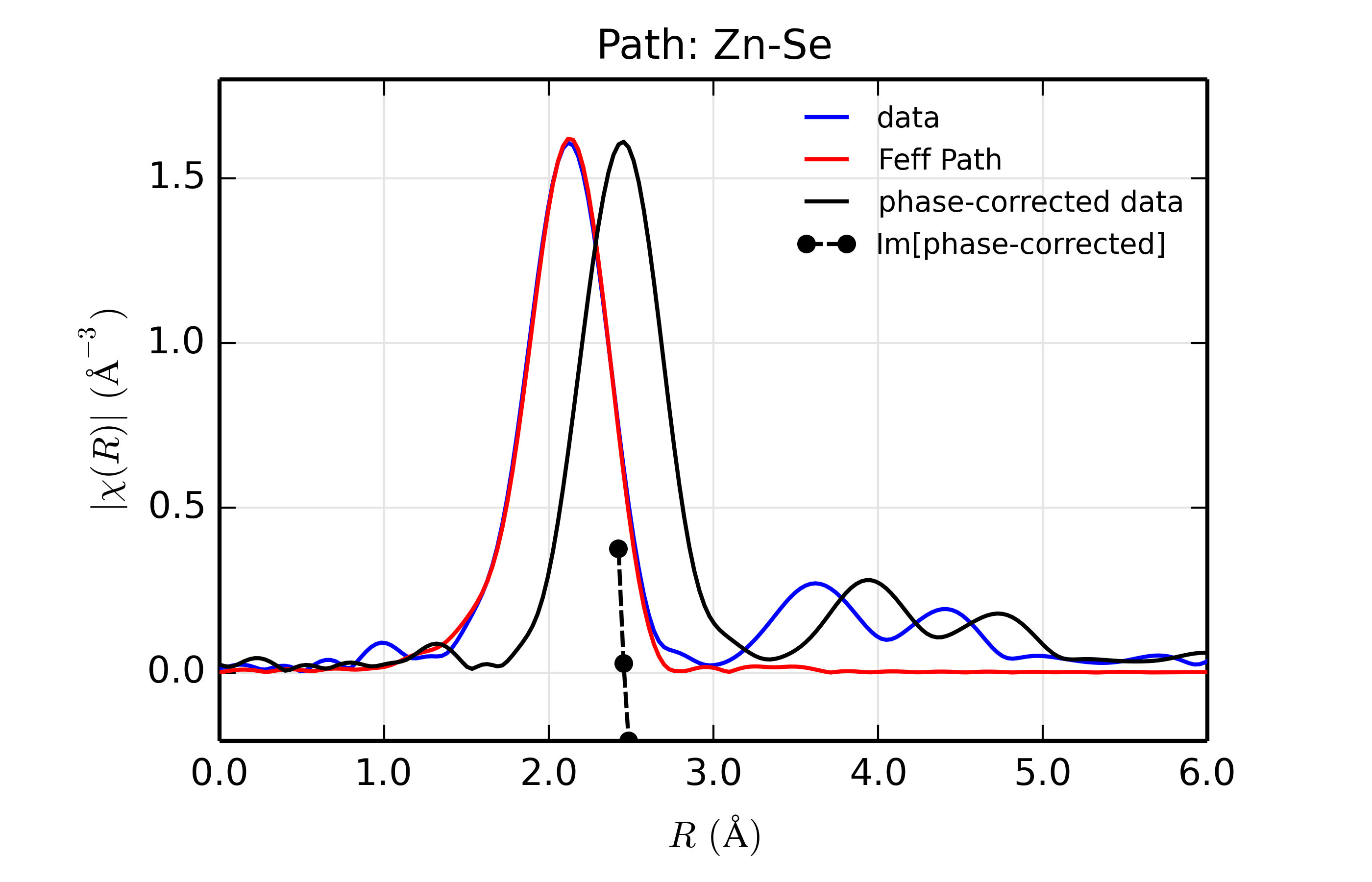
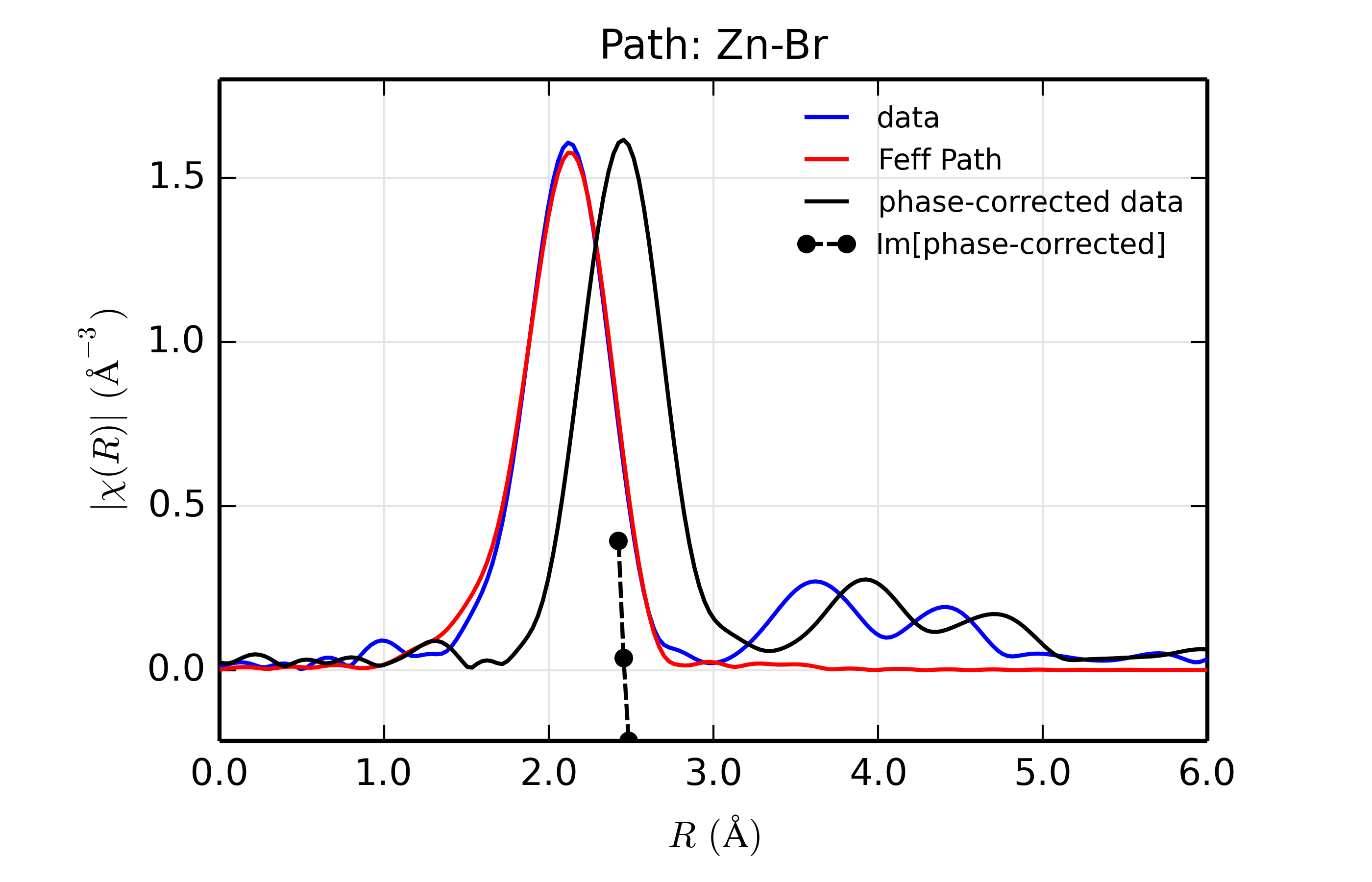
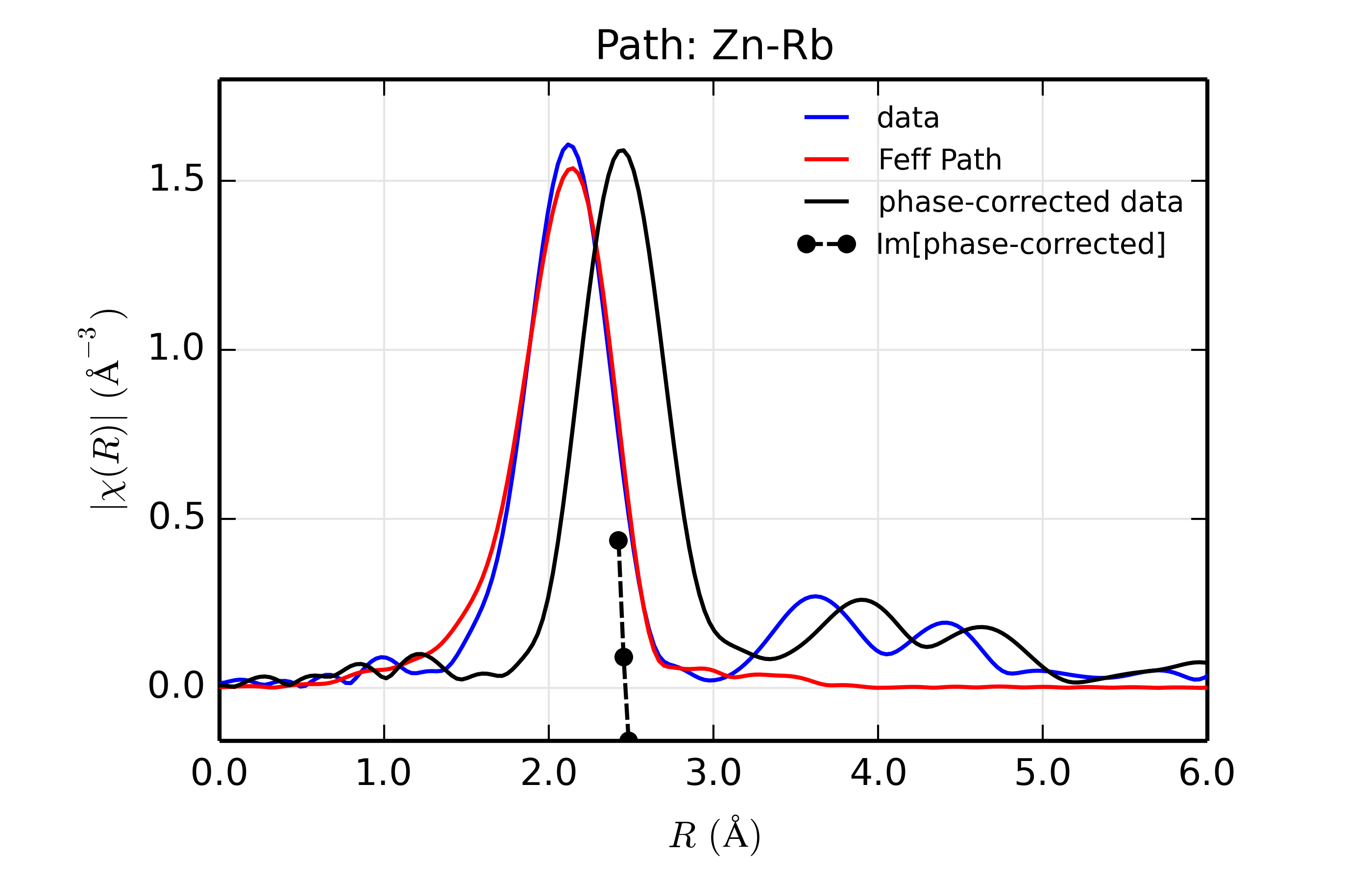
Figure 14.8.13.2 Fits to Zn K-edge of ZnSe with various atoms as the back-scatterer.
The figures also show phase-corrected Fourier transforms using the total
scattering phase from the Feff calculation to correct the data. This
correction is done in the phase_correct() procedure, where the data from
the feffNNNN.dat file (in the _feffdat group) is used to construct the
Feff phase shift (\(\delta(k)\) in the EXAFS Equation of Section
The EXAFS Equation using Feff and FeffPath Groups), and apply it to the data. Because this uses
complex math, we use the xftf_fast() function to the complex Fourier
transform and build the magnitude of the transform explicitly.
The phase corrected transforms are shown in black in Figure 14.8.13.2, and show the key benefit of these transforms – the peak in the phase corrected \(\chi(R)\) peaks much closer to an \(R\) that is the bond distance (for Zn-Se, around 2.45 \(\rm\AA\)), whereas the normal XAFS Fourier transform peaks much lower. This suggests a further test on whether the bond distance and \(Z\) of the scattering atom are correct. That is, in order for the phase-correction to give the correct interatomic distance, the total phase-shift has to be correct, which means that the \(Z\) for the scatterer has to be correct (see the EXAFS Equation in Section The EXAFS Equation using Feff and FeffPath Groups). So, we can compare the refined distance with the peak in the phase-corrected transform – if they agree, it gives good confidence that the scatterer is correct.
Since the spacing of points in \(R\) is \(\sim 0.03\rm\AA\), using the peak position may not be accurate enough. Instead, we can use the value where \(\rm Im[\chi(R)_{\rm{ph cor}}]\) passes through zero (see dashed lines in Figure 14.8.13.2 These values are reported in the Table of ZnSe Results as \(R_{\rm{phcor}}\).
We see an interesting trend that while the refined distance decreases with \(Z\), the value for \(R_{\rm{phcor}}\) increases slightly. The two values cross between Ge and Se. This is pretty good agreement, especially considering we left out the \(\sigma^2\) contribution to phase-shift in the EXAFS equation from this phase correction, and applied the theoretical phase-shift from Feff to the measured data. The \(Z\) dependence of \(R_{\rm{phcor}}\) is not as strong as the \(Z\) dependence of reduced chi-square, but this analysis also suggests that one can determine \(Z \pm 3\), at least in this rather favorable case.
Again, this is an unusually favorable case – a simple structure with a single well-isolated coordination shell. The phase-correction method will not work at all on a mixed coordination shell, and is likely to give larger errors for a highly-disordered system. But, for simple, well-characterized systems, the ability to do such analysis can be very powerful, and give increased confidence in the refined structure.