
16. X-ray Fluorescence Analysis
X-ray Fluorescence (XRF) Data can be manipulated, viewed, and analyzed with Larch. In this chapter, we’ll discuss how to transform data into Larch Groups of XRF data and how to use the Graphical visualization tool XRF Display to visualize and work with XRF spectr. We’ll also discuss how to analyze XRF spectra to quantify elemental compositions of samples. As part of that discussion of fitting XRF spectra, we’ll review some of the fundamental concepts of XRF Analysis and discuss how these features can affect the results of XRF analysis.
Since XRF spectra can be collected in as little as a few milliseconds with modern X-ray sources and solid-state detectors, it is common to build 2- or even 3-dimensional maps of XRF data, with each pixel in the map holding an XRF spectrum that can be analyzed. Larch’s GSE MapViewer is designed to work with and display such XRF maps, and to support the quantitative XRF analysis shown here.
A basic XRF spectrum from a solid-state detector – a silicon drift detector – as displayed in the XRF Display program is shown below. The spectrum consists of two arrays of a few thousand points: an energy array that holds energy at each point (or “channel”) in the array and a counts array that holds the counts in each channel.
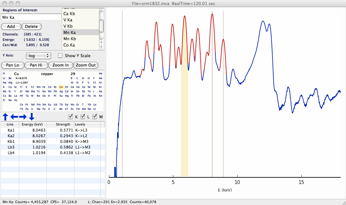
Figure 16.1 Typical X-ray fluorescence spectrum.
The peaks in this specra correpsond to characteristic X-ray emission lines from the elements. The presence of a particular peak in the spectrum indicates that the corresponding element was in the illuminated X-ray beam – the spectrum above indicates that Cu and Mn (and also Ca, V, and Co) are present in the sample. Furthermore, the intensity of each peak can be used to determine (or at least “infer”) the concentration of that particular element in the illuminated sample.
From a spectroscopic point-of-view XRF spectra are relatively easy to interpret: the characteristic emission energies for each atom are well known to high precision and the absorption and emission probabilities are known to pretty good precision (though perhaps only 10%). In this sense, a crude approach to XRF analysis is to use the area under the appropriate peaks as a quantifiable value for the elements abundance. This should definitely be taken as a rough approximation. The complications preventing such a simle interpretion of XRF spectra are due mostly to:
1. Strong X-ray attenuation effects. The attenuation of X-rays goes approximately as \(\mu \sim Z^4E^{-3}\), which is to say it has extremely high and non-linear dependence on the atomic number Z of the elements in the X-ray beam, and extremely high and non-linear dependence on the X-ray energy.
2. Overlaps of elemental peaks. That is, the emission energies for each element are known, but not unique. Each element will have multiple series of lines (K, L, M, etc), and these can be close enough in energy to cause some uncertainty in which elements are present.
3. Detector artefacts. Even the best energy-discriminating detectors used for most XRF analysis are limited in the resolution with which they can determine an X-ray energy. They also need some finite time (\(100ns\) to \(10{\mu}s\)) to count each X-ray and so have a “dead time” and can suffer from “pileup” that can distort the spectra.
These effects are understood pretty well and can mostly be compensated for in a thorough analysis, as will be discussed in more detail below. Importantly, together they means that simply taking the area under a portion of the curve in the XRF spectrum is generally not a good measure of the absolute abundance of an atom in the illuminated sample. In limited cases, where the bulk of the sample composition does change much, where peak overlaps are small, and where the detector is not saturated, the integrated intensities of selected peaks can be a good relative measure of elemental abundance.