\(\newcommand{\AA}{\unicode{x212B}}\)

14.2. XAFS: Pre-edge Subtraction, Normalization, and data treatment

After reading in data and constructing \(\mu(E)\), the principle pre-processing steps for XAFS analysis are pre-edge subtraction and normalization. Reading data and constructing \(\mu(E)\) are handled by internal larch functions, especially read_ascii(). The main XAFS-specific function for pre-edge subtraction and normalization is pre_edge().

This chapter also describes methods for the treatment of XAFS and XANES data including corrections for over-absorption (sometimes confusingly called self-absorption) and for spectral convolution and de-convolution.

14.2.1. The find_e0() function

larch.xafs.find_e0(*args, **kwargs)

calculate E0, the energy threshold of absorption, or ‘edge energy’, given mu(E).

E0 is found as the point with maximum derivative with some checks to avoid spurious glitches.

Parameters:

• energy (ndarray or group) – array of x-ray energies, in eV, or group

• mu (ndaarray or None) – array of mu(E) values

• group (group or None) – output group

• _larch (larch instance or None) – current larch session.

Returns:

Value of e0. If a group is provided, group.e0 will also be set.

Return type:

float

Notes

1. Supports First Argument Group convention convention, requiring group members energy and mu

2. Supports group argument and _sys.xafsGroup convention within Larch or if _larch is set.

14.2.2. The pre_edge() function

pre_edge(energy, mu, group=None, e0=None, step=None, pre1=None, pre2=None, norm1=None, norm2=None, nnorm=None, nvict=0)

Pre-edge subtraction and normalization. This performs a number of steps:

1. determine \(E_0\) (if not supplied) from max of deriv(mu)

2. fit a line of polynomial to the region below the edge

3. fit a polynomial to the region above the edge

4. extrapolate the two curves to \(E_0\) to determine the edge jump

Parameters:

• energy – 1-d array of x-ray energies, in eV

• mu – 1-d array of \(\mu(E)\)

• group – output group

• e0 – edge energy, \(E_0\) in eV. If None, it will be found.

• step – edge jump. If None, it will be found here.

• pre1 – low E range (relative to E0) for pre-edge fit. See Notes.

• pre2 – high E range (relative to E0) for pre-edge fit. See Notes.

• norm1 – low E range (relative to E0) for post-edge fit. See Notes.

• norm2 – high E range (relative to E0) for post-edge fit. See Notes.

• nnorm – degree of polynomial (ie, norm+1 coefficients will be found) for post-edge normalization curve. See Notes.

• nvict – energy exponent to use. See Notes.

• make_flat – boolean (Default True) to calculate flattened output.

Returns:

None.

Follows the First Argument Group convention, using group members named energy and mu. The following data is put into the output group:

attribute	meaning
e0	energy origin
edge_step	edge step
norm	normalized mu(E) (array)
flat	flattened, normalized mu(E) (array)
pre_edge	pre-edge curve (array)
post_edge	post-edge, normalization curve (array)
pre_slope	slope of pre-edge line
pre_offset	offset of pre-edge line
nvict	value of nvict used
nnorm	value of nnorm used
norm_c0	constant of normalization polynomial
norm_c1	linear coefficient of normalization polynomial
norm_c2	quadratic coefficient of normalization polynomial
norm_c*	higher power coefficients of normalization polynomial

For the pre-edge portion of the spectrum, a line is fit to \(\mu(E) E^{\rm{nvict}}\) in the region \(E={\rm{[e0+pre1, e0+pre2]}}\). pre1 and pre2 default to None, which will set:

• pre1 = e0 - 2nd energy point

• pre2 = roughly pre1/3.0, rounded to 5 eV steps

For the post-edge, a polynomial of order nnorm is fit to \(\mu(E) E^{\rm{nvict}}\) in the region \(E={\rm{[e0+norm1, e0+norm2]}}\). norm1, norm2, and nnorm default to None, which will set:

• norm2 = max energy - e0

• norm1 = roughly norm2/3.0, rounded to 5 eV

The value for nnorm = 2 if norm2-norm1>350, 1 if norm2-norm1>50, or 0 if less.

The “flattened” \(\mu(E)\) is found by fitting a quadratic curve (no matter the value of nnorm) to the post-edge normalized \(\mu(E)\) and subtracts that curve from it.

14.2.3. Pre-Edge Subtraction Example

A simple example of pre-edge subtraction:

# Larch
fname = 'fe2o3_rt1.xmu'
dat = read_ascii(fname, labels='energy mu i0')

pre_edge(dat, group=dat)

plot_mu(dat, show_pre=True, show_post=True)

or in plain Python:

from larch.io import read_ascii
from larch.xafs import pre_edge
from wxmplot.interactive import plot

fname = 'fe2o3_rt1.xmu'
dat = read_ascii(fname, labels='energy mu i0')

pre_edge(dat, group=dat)

plot(dat.energy, dat.mu, label='mu', xlabel='Energy (eV)',
     title=fname,show_legend=True)
plot(dat.energy, dat.pre_edge, label='pre-edge line')
plot(dat.energy, dat.post_edge, label='post-edge curve')

gives the following results:

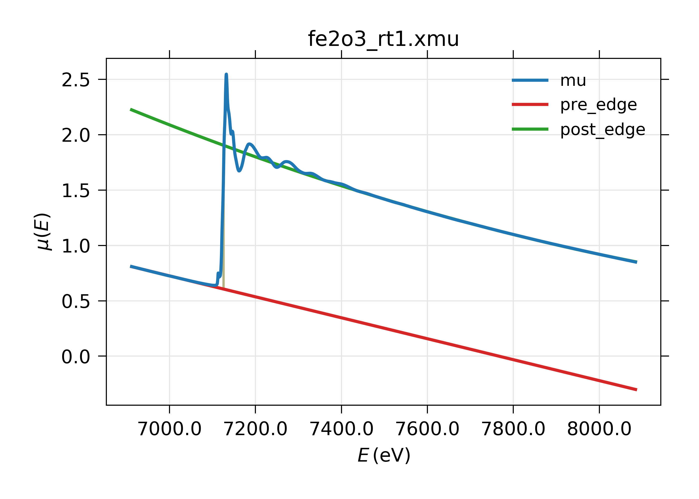
Figure 14.2.3.1 XAFS Pre-edge subtraction.

14.2.4. The MBACK algorithm

Larch provides an implementation of the MBACK algorithm of Weng [Weng, Waldo, and Penner-Hahn (2005)] with an option of using the modification proposed by Lee et al [Lee et al. (2009)]. In MBACK, the data are matched to the tabulated values of the imaginary part of the energy-dependent correction to the Thompson scattering factor, \(f''(E)\). To account for any instrumental or sample-dependent aspects of the shape of the measured data, \(\mu_{data}(E)\), a Legendre polynomial of order \(m\) centered around the absorption edge is subtracted from the data. To account for the sort of highly non-linear pre-edge which often results from Compton scattering in the measurement window of an energy-discriminating detector, a complementary error function is added to the Legendre polynomial.

The form of the normalization function, then, is

\[\mu_{back}(E) = \left[\sum_0^m C_i(E-E_0)^i\right] + A\cdot\operatorname{erfc}\left((E-E_{em}\right)/\xi)\]

where \(A\), \(E_{em}\), and \(\xi\) are the amplitude, centroid, and width of the complementary error function and \(s\) is a scaling factor for the measured data. \(E_{em}\) is typically the centroid of the emission line for the measured edge. This results in a function of \(3+m\) variables (a tabulated value of \(E_{em}\) is used). The function to be minimized, then is

\[\frac{1}{n_1} \sum_{1}^{n_1} \left[\mu_{tab}(E) + \mu_{back}(E) + s\cdot\mu_{data}(E)\right]^2 + \frac{1}{n_2} \sum_{n_1+1}^{N} \left[\mu_{tab}(E) + \mu_{back}(E) + s\cdot\mu_{data}(E)\right]^2\]

To give weight in the fit to the pre-edge region, which typically has fewer measured points than the post-edge region, the weight is adjusted by breaking the minimization function into two regions: the \(n_1\) data points below the absorption edge and the \(n_2\) data points above the absorption edge. \(n_1+n_2=N\), where N is the total number of data points.

If this is used in publication, a citation should be given to Weng [Weng, Waldo, and Penner-Hahn (2005)].

mback(energy, mu, group=None, ...)

Match measured \(\mu(E)\) data to tabulated cross-section data.

Parameters:

• energy – 1-d array of x-ray energies, in eV

• mu – 1-d array of \(\mu(E)\)

• group – output group

• z – the Z number of the absorber

• edge – the absorption edge, usually ‘K’ or ‘L3’

• e0 – edge energy, \(E_0\) in eV. If None, the tabulated value is used.

• leexiang – flag for using the use the Lee&Xiang extension [False]

• tables – ‘CL’ (Cromer-Liberman) or ‘Chantler’, [‘Chantler’]

• fit_erfc – if True, fit the amplitude and width of the complementary error function [False]

• return_f1 – if True, put f1 in the output group [False]

• pre_edge_kws – dictionary containing keyword arguments to pass to pre_edge().

Pre1:

low E range (relative to e0) for pre-edge region.

Pre2:

high E range (relative to e0) for pre-edge region.

Norm1:

low E range (relative to e0) for post-edge region.

Norm2:

high E range (relative to e0) for post-edge region.

Order:

order of the legendre polynomial for normalization.

Returns:

None.

Follows the First Argument Group convention, using group members named energy and mu. The following data is put into the output group:

attribute	meaning
fpp	matched \(\mu(E)\) data
f2	tabulated \(f''(E)\) data
f1	tabulated \(f'(E)\) data (if return_f1 is True)
mback_params	params group for the MBACK minimization function

Notes:

• The order parameter is the order of the Legendre polynomial. Data measured over a very short data range are likely best processed with order=2. Extended XAS data are often better processed with a value of 3 or 4. The order is enforced to be an integer between 1 and 6.

• A call to pre_edge() is made if e0 is not supplied.

• The option to return \(f'(E)\) is used by diffkk().

Here is an example of processing XANES data measured over an extended data range. This example is the K edge of copper foil, with the result shown in Figure 14.2.4.1.

from larch.io import read_ascii
from larch.xafs import mback
from wxmplot.interactive import plot

data = read_ascii('../xafsdata/cu_10k.xmu')
mback(data.energy, data.mu, group=a, z=29, edge='K', order=4)
plot(data.energy, data.f2, xlabel='Energy (eV)', ylabel='matched absorption', label='$f_2$',
     legend_loc='lr', show_legend=True)
plot(data.energy, data.fpp, label='Copper foil')

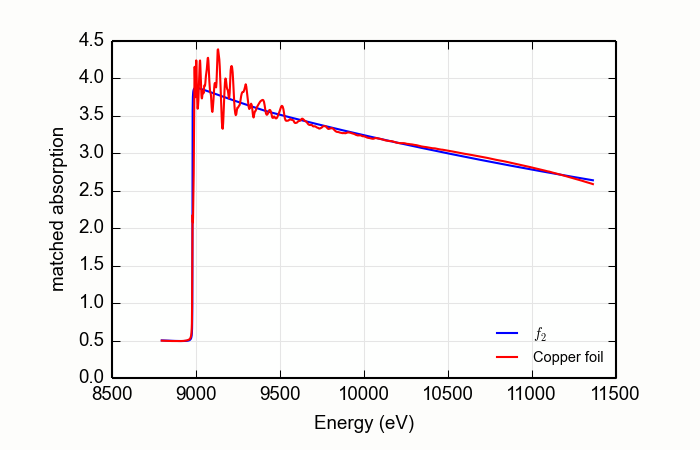
Figure 14.2.4.1 Using MBACK to match Cu K edge data measured on a copper foil.

Here is an example of processing XANES data measured over a rather short data range. This example is the magnesium silicate mineral talc, Mg₃Si₄O₁₀(OH)₂, measured at the Si K edge, with the result shown in Figure 14.2.4.2. Note that the order of the Legendre polynomial is set to 2 and that the whiteline parameter is set to avoid the large features near the edge.

data=read_ascii('Talc.xmu')
mback(data.e, data.xmu, group=a, z=14, edge='K', order=2, whiteline=50, fit_erfc=True)
newplot(data.e, data.f2, xlabel='Energy (eV)', ylabel='matched absorption', label='$f_2$',
        legend_loc='lr', show_legend=True)
plot(data.e, data.fpp, label='Talc ($\mathrm{Mg}_3\mathrm{Si}_4\mathrm{O}_{10}\mathrm{(OH)}_2$)')

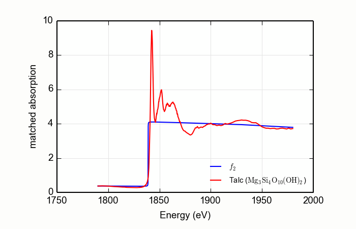
Figure 14.2.4.2 Using MBACK to match Si K edge data measured on talc.

mback_norm(energy, mu, group=None, ...)

A simplified version of mback() to normalize \(\mu(E)\) data to tabulated cross-section data for \(f''(E)\).

Returns:

group.norm_poly: normalized mu(E) from pre_edge() group.norm: normalized mu(E) from this method group.mback_mu: tabulated f2 scaled and pre_edge added to match mu(E) group.mback_params: Group of parameters for the minimization

References:

• MBACK (Weng, Waldo, Penner-Hahn): https://dx.doi.org/10.1086/303711

• Chantler: https://dx.doi.org/10.1063/1.555974

Parameters:

• energy – 1-d array of x-ray energies, in eV

• mu – 1-d array of \(\mu(E)\)

• group – output group

• z – the Z number of the absorber

• edge – the absorption edge, usually ‘K’ or ‘L3’

• e0 – edge energy, \(E_0\) in eV. If None, the tabulated value is used.

• pre1 – low E range (relative to E0) as for pre_edge().

• pre2 – high E range (relative to E0) as for pre_edge().

• norm1 – low E range (relative to E0) as for pre_edge().

• norm2 – high E range (relative to E0) as for pre_edge().

• nnorm – degree of polynomial as for pre_edge().

Follows the First Argument Group convention, using group members named energy and mu. The following data is put into the output group:

attribute	meaning
norm_poly	normalized \(\mu(E)\) from pre_edge().
norm	normalized \(\mu(E)\) from this method/
mback_mu	tabulated \(f'(E)\) scaler and pre-edge added
mback_params	params group for the MBACK minimization function

14.2.5. Pre-edge baseline subtraction

A common application of XAFS is the analysis of “pre-edge peaks” of transition metal oxides to determine oxidation state and molecular configuration. These peaks sit just below the main absorption edge (typically, due to metal 4p electrons) of a main K edge, and are due to overlaps of the metal d-electrons and oxygen p-electrons, and are often described in terms of molecular orbital theory.

To analyze the energies and relative strengths of these pre-edge peaks, it is necessary to try to remove the contribution of the main edge. The main edge (or at least its low energy side) can be modeled reasonably well as a Lorentzian function for these purposes of describing the tail below the pre-edge peaks.

larch.xafs.prepeaks_setup(*args, **kwargs)

set up pre edge peak group.

This assumes that pre_edge() has been run successfully on the spectra and that the spectra has decent pre-edge subtraction and normalization.

Parameters:

• energy (ndarray or group) – array of x-ray energies, in eV, or group (see note 1)

• norm (ndarray or None) – array of normalized mu(E) to be fit (deprecated, see note 2)

• arrayname (string or None) – name of array to use as data (see note 2)

• group (group or None) – output group

• emax (float or None) – max energy (eV) to use for baesline fit [e0-5]

• emin (float or None) – min energy (eV) to use for baesline fit [e0-40]

• elo – (float or None) low energy of pre-edge peak region to not fit baseline [e0-20]

• ehi – (float or None) high energy of pre-edge peak region ot not fit baseline [e0-10]

• _larch (larch instance or None) – current larch session.

A group named prepeaks will be created in the output group, containing:

attribute	meaning
energy	energy array for pre-edge peaks = energy[emin:emax]
norm	spectrum over pre-edge peak energies

Note that ‘norm’ will be used here even if a differnt input array was used.

Notes

1. Supports First Argument Group convention convention, requiring group members energy and norm

2. You can pass is an array to fit with ‘norm=’, or you can name the array to use with arrayname, which can be one of [‘norm’, ‘flat’, ‘deconv’, ‘aspassed’, None] with None and ‘aspassed’ meaning that the argument of norm will be used, as passed in.

3. Supports group argument and _sys.xafsGroup convention within Larch or if _larch is set.

larch.xafs.pre_edge_baseline(*args, **kwargs)

remove baseline from main edge over pre edge peak region

This assumes that pre_edge() has been run successfully on the spectra and that the spectra has decent pre-edge subtraction and normalization.

Parameters:

• energy (ndarray or group) – array of x-ray energies, in eV, or group (see note 1)

• norm (ndarray or group) – array of normalized mu(E)

• group (group or None) – output group

• elo (float or None) – low energy of pre-edge peak region to not fit baseline [e0-20]

• ehi (float or None) – high energy of pre-edge peak region ot not fit baseline [e0-10]

• emax (float or None) – max energy (eV) to use for baesline fit [e0-5]

• emin (float or None) – min energy (eV) to use for baesline fit [e0-40]

• form (string) – form used for baseline (see description) [‘linear+lorentzian’]

• _larch (larch instance or None) – current larch session.

A function will be fit to the input mu(E) data over the range between [emin:elo] and [ehi:emax], ignorng the pre-edge peaks in the region [elo:ehi]. The baseline function is specified with the form keyword argument, which can be one or a combination of ‘lorentzian’, ‘gaussian’, or ‘voigt’, plus one of ‘constant’, ‘linear’, ‘quadratic’, for example, ‘linear+lorentzian’, ‘constant+voigt’, ‘quadratic’, ‘gaussian’.

A group named ‘prepeaks’ will be used or created in the output group, containing

attribute	meaning
energy	energy array for pre-edge peaks = energy[emin:emax]
baseline	fitted baseline array over pre-edge peak energies
norm	spectrum over pre-edge peak energies
peaks	baseline-subtraced spectrum over pre-edge peak energies
centroid	estimated centroid of pre-edge peaks (see note 3)
peak_energies	list of predicted peak energies (see note 4)
fit_details	details of fit to extract pre-edge peaks.

Notes

1. Supports First Argument Group convention convention, requiring group members energy and norm

2. Supports group argument and _sys.xafsGroup convention within Larch or if _larch is set.

3. The value calculated for prepeaks.centroid will be found as (prepeaks.energy*prepeaks.peaks).sum() / prepeaks.peaks.sum()

4. The values in the peak_energies list will be predicted energies of the peaks in prepeaks.peaks as found by peakutils.

14.2.6. Over-absorption Corrections

For XAFS data measured in fluorescence, a common problem of over-absorption in which too much of the total X-ray absorption coefficient is from the absorbing element. In such cases, the implicit assumption in a fluorescence XAFS measurement that the fluorescence intensity is proportional to the absorption coefficient of the element of interest breaks down. This is often referred to as self-absorption in the older XAFS literature, but the term should be avoided as it is quite a different effect from self-absorption in X-ray fluorescence analysis. In fact, the effect is more like extinction in that the fluorescence probability approaches a constant, with no XAFS oscillations, as the total absorption coefficient is dominated by the element of interest. Over-absorption most strongly effects the XAFS oscillation amplitude, and so coordination number and mean-square displacement parameters in the EXAFS, and edge-position and pre-edge peak height for XANES. Fortunately, the effect can be corrected for small over-absorption.

For XANES, a common correction method from the FLUO program by D. Haskel ([Haskel (1999)]) can be used. The algorithm is contained in the fluo_corr() function.

fluo_corr(energy, mu, formula, elem, group=None, edge='K', anginp=45, angout=45, **pre_kws)

calculate \(\mu(E)\) corrected for over-absorption in fluorescence XAFS using the FLUO algorithm (suitable for XANES, but questionable for EXAFS).

Parameters:

• energy – 1-d array of x-ray energies, in eV

• mu – 1-d array of \(\mu(E)\)

• formula – string for sample stoichiometry

• group – output group

• elem – atomic symbol (‘Zn’) or Z of absorbing element

• edge – name of edge (‘K’, ‘L3’, …) [default ‘K’]

• anginp – input angle in degrees [default 45]

• angout – output angle in degrees [default 45]

• pre_kws – additional keywords for pre_edge().

Returns:

None

Follows the First Argument Group convention, using group members named energy and mu. The value of mu_corr and norm_corr will be written to the output group, containing \(\mu(E)\) and normalized \(\mu(E)\) corrected for over-absorption.

14.2.7. Spectral deconvolution

In order to readily compare XAFS data from different sources, it is sometimes necessary to consider the energy resolution used to collect each spectum. To be clear, the resolution of an EXAFS spectrum includes contributions from the x-ray sources, instrumental broadening from the x-ray optics (especially the X-ray monochromator used in most measurements), and the intrinsic lifetime of the excited core electronic level. For data measured in X-ray fluorescence or electron emission mode, the energy resolution can also includes the energy width of the decay channels measured.

For a large fraction of XAFS data, the energy resolution is dominated by the intrinsic width of the excited core level and by the resolution of a silicon (111) double crystal monochromator, and so does not vary appreciably between spectra taken at different facilities or at different times. Exceptions to this rule occur when using a higher order reflection of a silicon monochromator or a different monochromator altogether. Resolution can also be noticeably worse for data taken at older (first and second generation) sources and beamlines, either without a collimating mirror or slits before the monochromator to improve the resolution. In addition, high-resolution X-ray fluorescence measurements can be used to dramatically enhance the energy resolution of XAFS spectra, and are becoming widely available.

Because of these effects, it is sometimes useful to change the resolution of XAFS spectra. For example, one may need to reduce the resolution to match data measured with degraded resolution. This can be done with xas_convolve() which convolves an XAFS spectrum with either a Gaussian or Lorentzian function with a known energy width. Note that convolving with a Gaussian is less dramatic than using a Lorentzian, and usually better reflects the effect of an incident X-ray beam with degraded resolution due to source or monochromator.

One may also want to try to improve the energy resolution of an XAFS spectrum, either to compare it to data taken with higher resolution or to better identify and enumerate peaks in a XANES spectrum. This can be done with xas_deconvolve() function which de-convolves either a Gaussian or Lorentzian function from an XAFS spectrum. This usually requires fairly good data. Whereas a Gaussian most closely reflects broadening from the X-ray source, broadening due to the natural energy width of the core levels is better described by a Lorentzian. Therefore, to try to reduce the influence of the core level in order better mimic high-resolution fluorescence data, de-convolving with a Lorentzian is often better.

14.2.7.1. xas_convolve()

xas_convolve(energy, norm=None, group=None, form='lorentzian', esigma=1.0, eshift=0.0):

convolve a normalized mu(E) spectra with a Lorentzian or Gaussian peak shape, degrading separation of XANES features.

This is provided as a complement to xas_deconvolve, and to deliberately broaden spectra to compare with spectra measured at lower resolution.

Parameters:

• energy – 1-d array of \(E\)

• norm – 1-d array of normalized \(\mu(E)\)

• group – output group

• form – form of deconvolution function. One of ‘lorentzian’ or ‘gaussian’ [‘lorentzian’]

• esigma – energy \(\sigma\) (in eV) to pass to gaussian() or lorentzian() lineshape [1.0]

• eshift – energy shift (in eV) to apply to result. [0.0]

Follows the First Argument Group convention, using group members named energy and norm. The following data is put into the output group:

attribute	meaning
conv	array of convolved, normalized \(\mu(E)\)

14.2.7.2. xas_deconvolve()

xas_deconvolve(energy, norm=None, group=None, form='lorentzian', esigma=1.0, eshift=0.0, smooth=True, sgwindow=None, sgorder=3)

XAS spectral deconvolution

de-convolve a normalized mu(E) spectra with a peak shape, enhancing the intensity and separation of peaks of a XANES spectrum.

The results can be unstable, and noisy, and should be used with caution!

Parameters:

• energy – 1-d array of \(E\)

• norm – 1-d array of normalized \(\mu(E)\)

• group – output group

• form – form of deconvolution function. One of ‘lorentzian’ or ‘gaussian’ [‘lorentzian’]

• esigma – energy \(\sigma\) (in eV) to pass to gaussian() or lorentzian() lineshape [1.0]

• eshift – energy shift (in eV) to apply to result. [0.0]

• smooth – whether to smooth the result with the Savitzky-Golay method [True]

• sgwindow – window size for Savitzky-Golay function [found from data step and esigma]

• sgorder – order for the Savitzky-Golay function [3]

Follows the First Argument Group convention, using group members named energy and norm.

Smoothing with savitzky_golay() requires a window and order. By default, window = int(esigma / estep) where estep is step size for the gridded data, approximately the finest energy step in the data.

The following data is put into the output group:

attribute	meaning
deconv	array of deconvolved, normalized \(\mu(E)\)

14.2.7.3. Examples using xas_deconvolve() and xas_convolve()

An example using xas_deconvolve() to deconvolve a XAFS spectrum would be:

## examples/xafs/doc_deconv1.lar
dat = read_ascii('../xafsdata/fe2o3_rt1.xmu', labels='energy mu i0')

pre_edge(dat)
xas_deconvolve(dat, esigma=1.0)

plot_mu(dat, show_norm=True, emin=-30, emax=70)
plot(dat.energy, dat.deconv, label='deconvolved')

## end of examples/xafs/doc_deconv1.lar

resulting in deconvolved data:

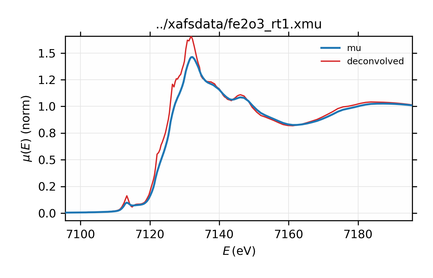
Figure 14.2.7.1 Deconvolved XAFS spectrum for \(\rm Fe_2O_3\).

To de-convolve an XAFS spectrum using the energy width of the core level, we can use the _xray.core_width() function, as shown below for Cu metal. We can also test that the deconvolution is correct by using xas_convolve() to re-convolve the result and comparing it to original data. This can be done with:

## examples/xafs/doc_deconv2.lar

dat = read_ascii('../xafsdata/cu_metal_rt.xdi', labels='energy i0 i1 mu')
dat.mu = -log(dat.i1 / dat.i0)

pre_edge(dat)

esigma = core_width('Cu', edge='K')

xas_deconvolve(dat, esigma=esigma)

plot_mu(dat, show_norm=True, emin=-50, emax=250)
plot(dat.energy, dat.deconv, label='deconvolved')

# Test convolution:
test = group(energy=dat.energy, norm=dat.deconv)
xas_convolve(test, esigma=esigma)
plot_mu(dat, show_norm=True, emin=-50, emax=250, win=2)
plot(test.energy, 100*(test.conv-dat.norm),
     label='(reconvolved - original)x100', win=2)
## end of examples/xafs/doc_deconv2.lar

with results shown below:

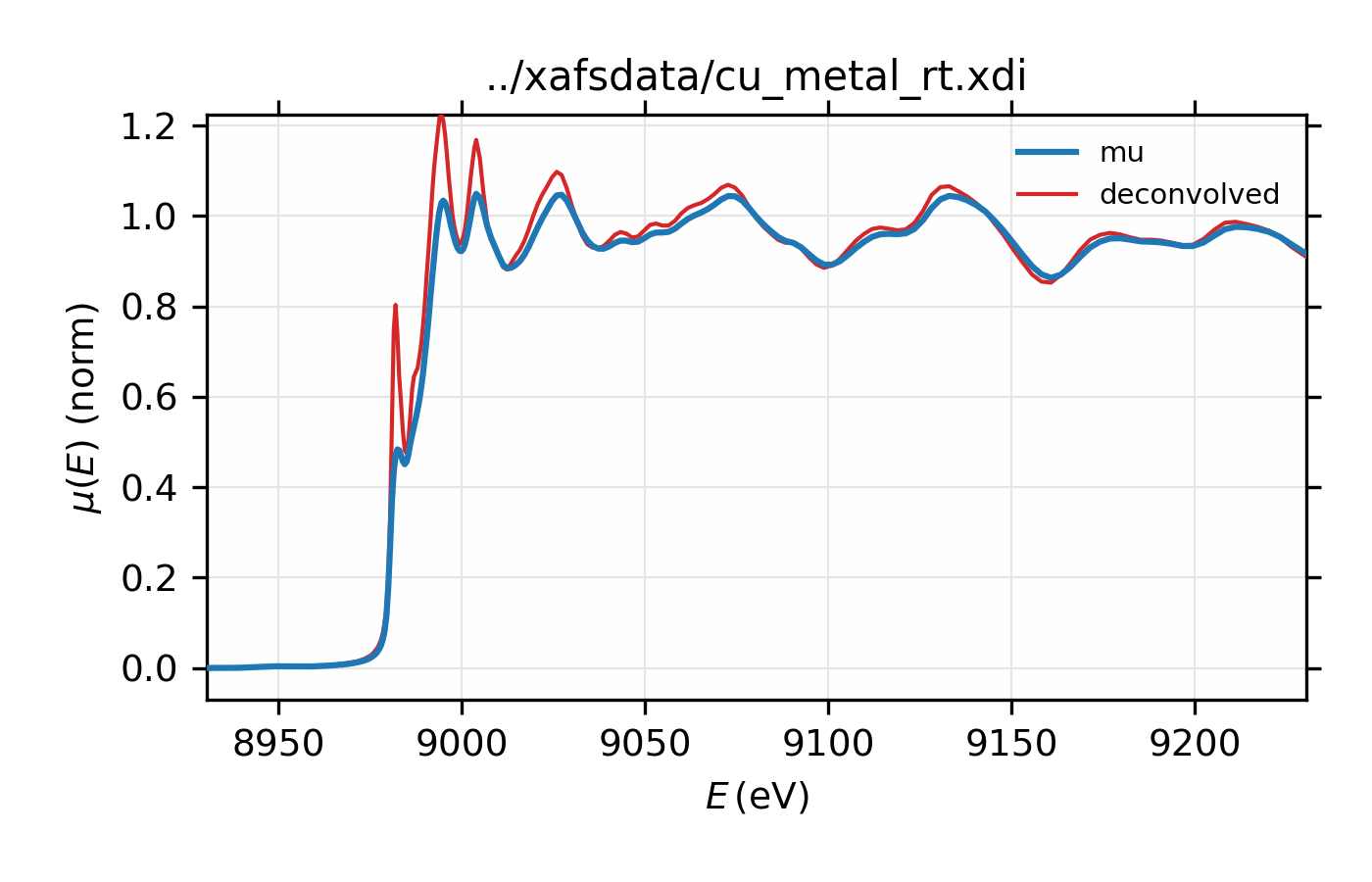
Figure 14.2.7.2 XAS for Cu metal normalized \(\mu(E)\) and spectrum deconvolved by the energy of its core level.

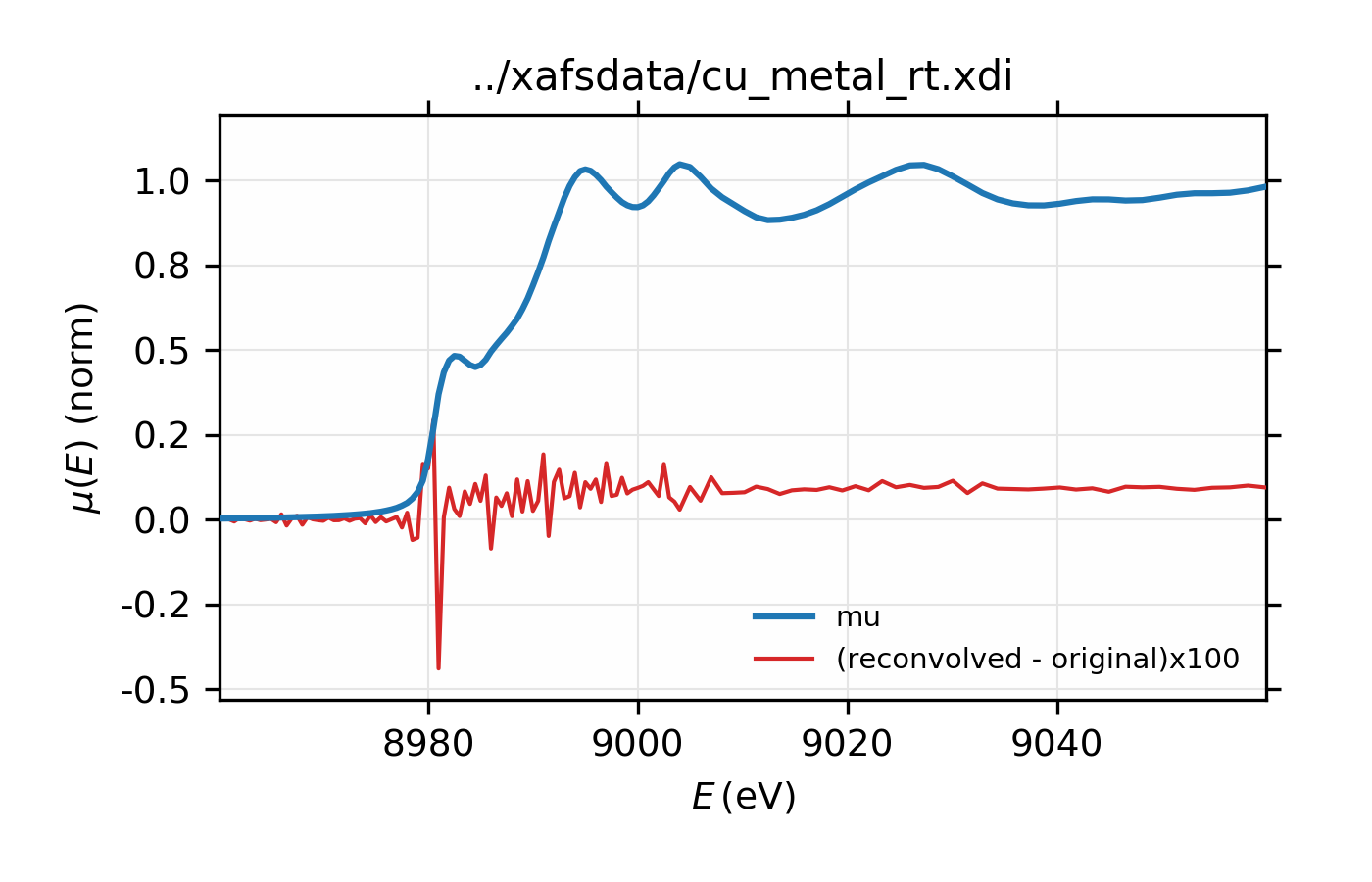
Figure 14.2.7.3 Comparison of original and re-convolved XAS spectrum for Cu metal. The difference shown in red is multiplied by 100.

Example of simple usage of xas_deconvolve() and xas_convolve() for Cu metal.

Finally, de-convolution of \(L_{\rm III}\) XAFS data can be particularly dramatic and useful. As with the copper spectrum above, we’ll deconvolve \(L_{\rm III}\) XAFS for platinum, using the nominal energy width of the core level (5.17 eV). For this example, we also see noticeable improvement in amplitude of the XAFS.

## examples/xafs/doc_deconv3.lar

data = read_ascii('../xafsdata/pt_metal_rt.xdi', labels='energy time i1 i0')
data.mu = -log(data.i1 / data.i0)

pre_edge(data)
autobk(data, rbkg=1.1, kweight=2)
xftf(data, kmin=2, kmax=17, dk=5, kwindow='kaiser', kweight=2)

xas_deconvolve(data, esigma=core_width('Pt', edge='L3'))

decon = group(energy=data.energy, mu=data.deconv, filename=data.filename)
autobk(decon, rbkg=1.1, kweight=2)
xftf(decon, kmin=2, kmax=17, dk=5, kwindow='kaiser', kweight=2)

# plot in E
plot_mu(data, show_norm=True, emin=-50, emax=250)
plot(data.energy, data.deconv, label='deconvolved',  win=1)

# plot in k
plot_chik(data, kweight=2, show_window=False, win=2)
plot_chik(decon, kweight=2, show_window=False,
          label='deconvolved', new=False, win=2)

# plot in R
plot_chir(data,  win=3)
plot_chir(decon, label='deconvolved', new=False, win=3)
## end examples/xafs/doc_deconv3.lar

with results shown below:

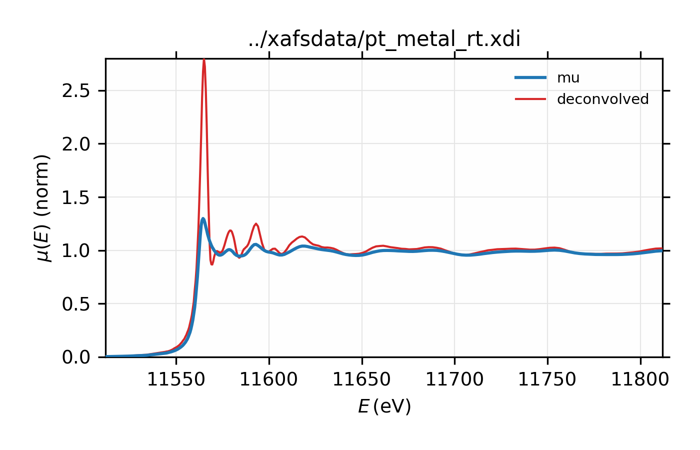
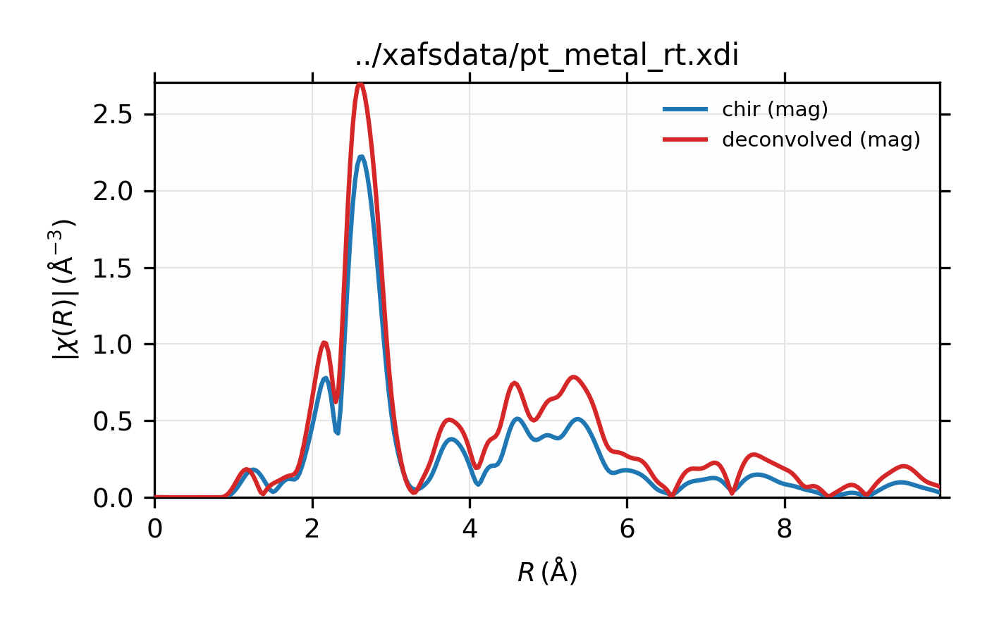
Example of simple usage of xas_deconvolve() and xas_convolve() for \(L_{\rm III}\) XAFS of Pt metal. \(L_{\rm III}\) XAFS of Pt metal, normalized \(\mu(E)\) for raw data and the spectrum deconvolved by the energy of its core level.