
13.6. Fit Examples
This section contains a few illustrative fitting examples. As mentioned earlier, the important pieces to have for a fit are:
1. a Parameter Group: a group that contains all the parameters (both truly variable parameters as well as any constrained parameters) for the fit.
2. an Objective Function that takes the Parameter Group as the first argument, and returns an array to be minimized in the least-squares sense.
The files for the examples shown here are all can be found in the examples/fitting folder of the main Larch distribution.
13.6.1. Example 1: Fitting a Simple Gaussian
Here we make a simple mock data set and fit a Gaussian function to it. Though a fairly simple example, and one that is guaranteed to work well, it touches on all the concepts discussed above, and is a reasonable representation of the sort of analysis actually done when modeling many kinds of data. The script to do the fit looks like this:
## examples/fitting/doc_example1.lar
# create mock data
mdat = group()
mdat.x = linspace(-10, 10, 201)
mdat.y = 1.0 + gaussian(mdat.x, amplitude=12, center=1.5, sigma=2.0) + \
         random.normal(size=len(mdat.x), scale=0.050)

# create a parameter group for the fit:
params = param_group(off = guess(0),
                     amp = guess(5, min=0),
                     cen = guess(2),
                     wid = guess(1, min=0))

init = params.off + gaussian(mdat.x, params.amp, params.cen, params.wid)

# define objective function for fit residual
def resid(p, data):
    return data.y - (p.off + gaussian(data.x, p.amp, p.cen, p.wid))
#enddef

# perform fit
out  = minimize(resid, params, args=(mdat,))

#
# make final array
final = params.off + gaussian(mdat.x, params.amp, params.cen, params.wid)
#
# plot results
plot(mdat.x, mdat.y, label='data', show_legend=True, new=True)
plot(mdat.x, init,   label='initial', color='black', style='dotted')
plot(mdat.x, final,  label='final', color='red')

# print report of parameters, uncertainties
print(fit_report(out))

## end of examples/fitting/doc_example1.lar
This fitting script consists of several components, which we’ll go over in some detail.
1 create mock data: Here we use the builtin
_math.gaussian()function to create the model function. We also add simulated noise to the model data with therandom.normal()function from numpy.2. create a group of fit parameters: Here we create a group with several components, all defined by the
_math.guess()function to create variable Parameters. Two of the parameters have a lower bound set. We also calculate the initial value for the model using the initial guesses for the parameter values.3. define objective function for fit residual: As above, this function will receive the group of fit parameters as the first argument, and may also receive other arguments as specified in the call to
_math.minimize(). This function returns the residual of the fit (data - model).4. perform fit. Here we call
_math.minimize()with arguments of the objective function, the parameter group, and any additional positional arguments to the objective function (keyword/value arguments can also be supplied). When this has completed, we calculate to model function with the final values of the parameters.5. plot results. Here we plot the data, starting values, and the final fit.
6. print report of parameters, uncertainties. Here we print out a report of the fit statistics, best fit values, uncertainties and correlations between variables.
The printed output from fit_report(params) will look like this:
[[Fit Statistics]]
    # function evals   = 28
    # data points      = 201
    # variables        = 4
    chi-square         = 0.53784
    reduced chi-square = 0.0027302
    Akaike info crit   = -1182.6
    Bayesian info crit = -1169.4
[[Variables]]
    amp:   11.9259429 +/- 0.078146 (0.66%) (init= 5)
    cen:   1.50726422 +/- 0.010365 (0.69%) (init= 2)
    off:   1.00495225 +/- 0.005356 (0.53%) (init= 0)
    wid:   1.99121482 +/- 0.012135 (0.61%) (init= 1)
[[Correlations]] (unreported correlations are <  0.100)
    C(amp, off)                  = -0.726
    C(amp, wid)                  =  0.717
    C(wid, off)                  = -0.520
And the plot of data and fit will look like this:
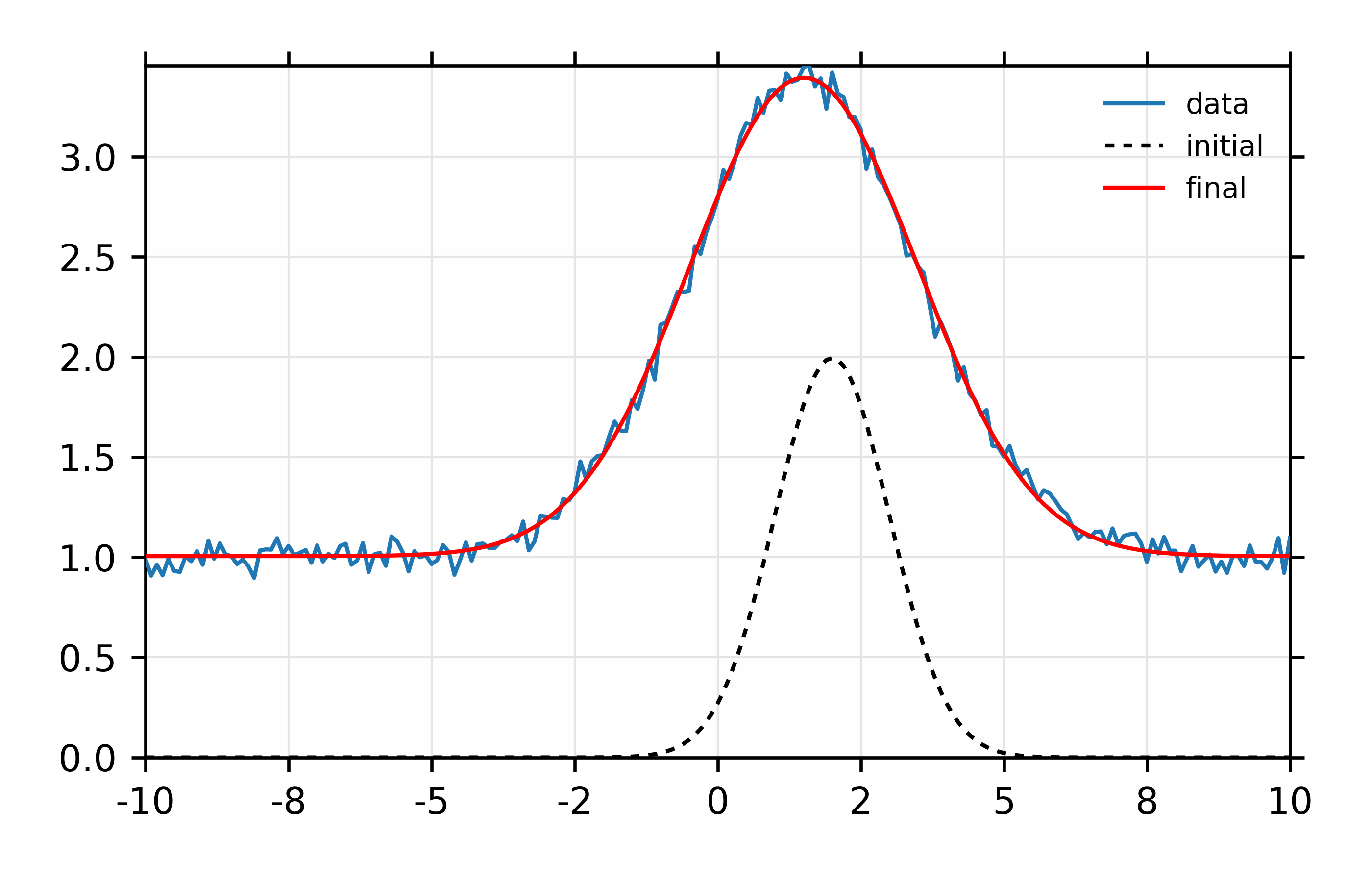
Figure 13.6.1.1 Simple fit to mock data
13.6.2. Example 2: Fitting XANES Pre-edge Peaks
This example extends on the previous one of fitting peaks. Though following the same basic approach (write an objective function, define parameters, perform fit), we add several steps that you might use when modeling real data:
using data read in from a text file,
using more lineshapes, here 3 peak-like functions and an error-function.
Consequently, the script is a bit longer:
## examples/fitting/doc_example2a.lar
# read data
dat = read_ascii('doc_example2.dat', labels='energy xmu i0')

# do pre-processing steps, here XAFS pre-edge removal
pre_edge(dat.energy, dat.xmu, group=dat)

# select data range to be considered in the fit here.
# note that this could be done inside the objective function,
# but doing these steps here means it done only once.
i1, i2 = index_of(dat.energy, 7105), index_of(dat.energy, 7125)
dat.e = dat.energy[i1+1:i2+1]
dat.y = dat.norm[i1+1:i2+1]

def make_model(pars, data, components=False):
    """make model of spectra: 2 peak functions, 1 erf function, offset"""
    p1 = gaussian(data.e, pars.amp1, pars.cen1, pars.wid1)
    p2 = gaussian(data.e, pars.amp2, pars.cen2, pars.wid2)

    e1 = pars.off + pars.erf_amp * erf( pars.erf_wid*(data.e - pars.erf_cen))
    sum = p1 + p2 + e1
    if components:
        return sum, p1, p2,  e1
    endif
    return sum
enddef

# create a parameter group for the fit:
params = param_group(
    cen1 = param(7113.25, vary=True, min=7111, max=7115),
    cen2 = param(7116.0, vary=True, min=7115, max=7120),

    amp1 = param(0.25, vary=True, min=0),
    amp2 = param(0.25, vary=True, min=0),

    wid1 = param(0.6, vary=True, min=0.05),
    wid2 = param(1.2, vary=True, min=0.05),

    off  = param(0.50, vary=True),

    erf_amp = param(0.50, vary=True),
    erf_wid = param(0.50, vary=True),
    erf_cen = param(7123.5, vary=True, min=7121, max=7124)
    )

def resid(pars, data):
    "fit residual"
    return make_model(pars, data) - data.y
enddef

mfit = minimize(resid, params, args=(dat,))

print( fit_report(mfit, show_correl=False))

# now plot results (2 different windows)
final, f1, f2, e1 = make_model(params, dat, components=True)
plot(dat.e, dat.y,  label='data', marker='+',
     show_legend=True, legend_loc='ul',
     xlabel='Energy (eV)', ylabel='$\\mu(E)$',
     title='Fe pre-edge peak-fit: best fit and residual',
     new=True)

plot(dat.e, final,  label='fit')
plot(dat.e, (final-dat.y)*10, label='diff (10x)')

plot(dat.e, dat.y, label='data', marker='+',
     show_legend=True, legend_loc='ul',
     xlabel='Energy (eV)', ylabel='$\\mu(E)$',
     title='Fe pre-edge peak-fit: components',
     new=True, win=2)

plot(dat.e, f1, label='peak1', win=2)
plot(dat.e, f2, label='peak2', win=2)
plot(dat.e, e1, label='erf +offset', win=2, color='red', style='dashed')

## end of examples/fitting/doc_example2a.lar
First, we read in the data and do some XAFS-specific preprocessing step.
Also note that we limit the range of the data from the full data set using
the index_of function. The objective function resid() is very
simple, calling make_models() which creates the model of two Gaussian
peaks, an error function, and an offset. There are 10 parameters for the
fit. We’re fitting the spectra with two Gaussian functions and an error
function. It is often observed that if the centroids of peak functions such
as Gaussians are left to vary completely freely they tend to wander around
and give lousy fits, so here we place fairly tight controls on the
centroids. We also place bounds on the amplitudes and widths of the peaks,
so they can’t go too far astray.
The fit gives a report (ignoring correlations) like this:
[[Fit Statistics]]
    # function evals   = 170
    # data points      = 51
    # variables        = 10
    chi-square         = 0.0012762
    reduced chi-square = 3.1126e-05
    Akaike info crit   = -520.38
    Bayesian info crit = -501.06
[[Variables]]
    amp1:      0.19742004 +/- 0.037564 (19.03%) (init= 0.25)
    amp2:      0.21393220 +/- 0.048193 (22.53%) (init= 0.25)
    cen1:      7113.28403 +/- 0.143034 (0.00%) (init= 7113.25)
    cen2:      7116.46195 +/- 0.279419 (0.00%) (init= 7116)
    erf_amp:   0.38223607 +/- 0.010433 (2.73%) (init= 0.5)
    erf_cen:   7122.29627 +/- 0.097868 (0.00%) (init= 7123.5)
    erf_wid:   0.27474480 +/- 0.011462 (4.17%) (init= 0.5)
    off:       0.39565509 +/- 0.010346 (2.62%) (init= 0.5)
    wid1:      1.07507112 +/- 0.105954 (9.86%) (init= 0.6)
    wid2:      1.58457992 +/- 0.307342 (19.40%) (init= 1.2)
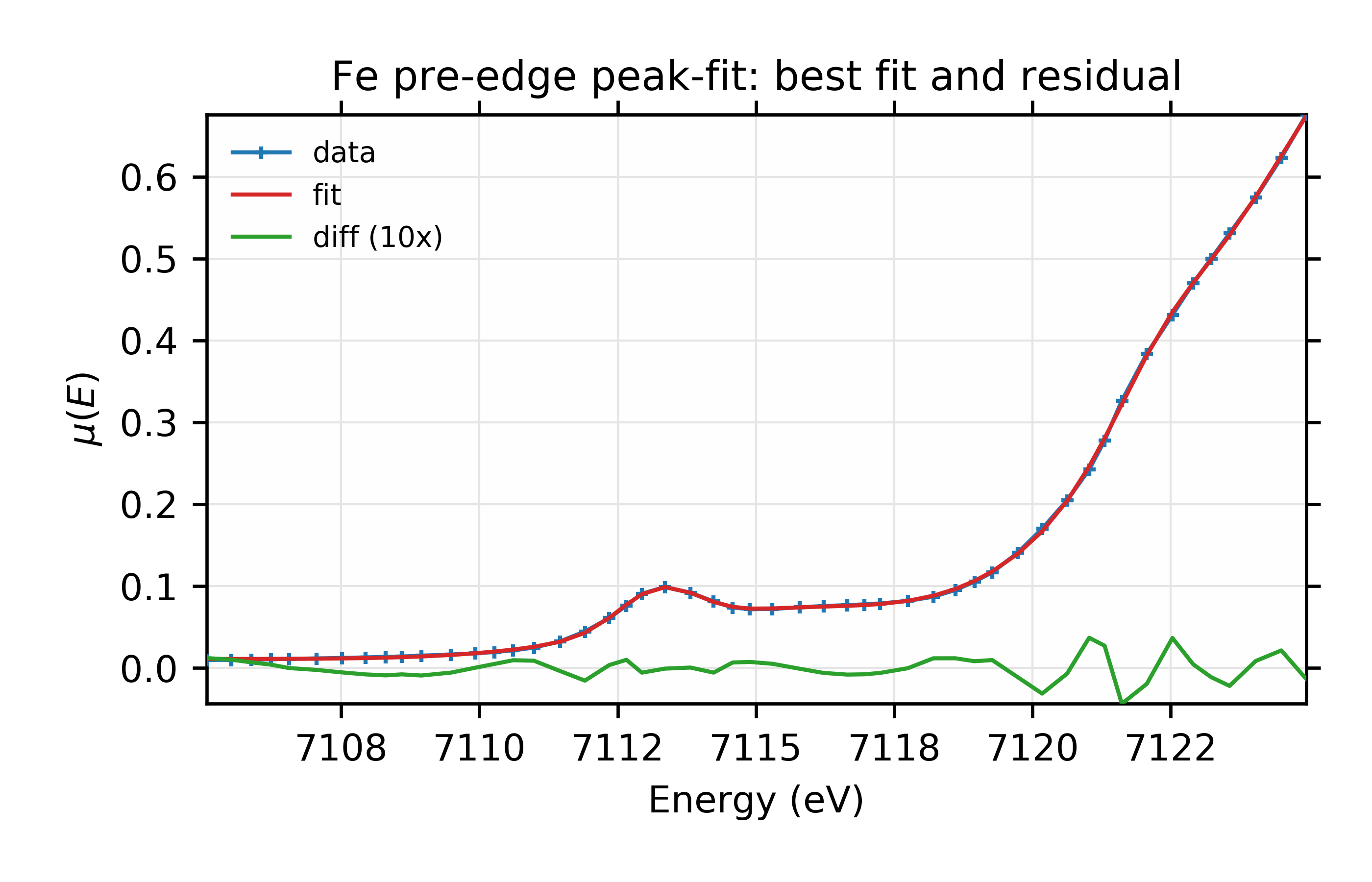
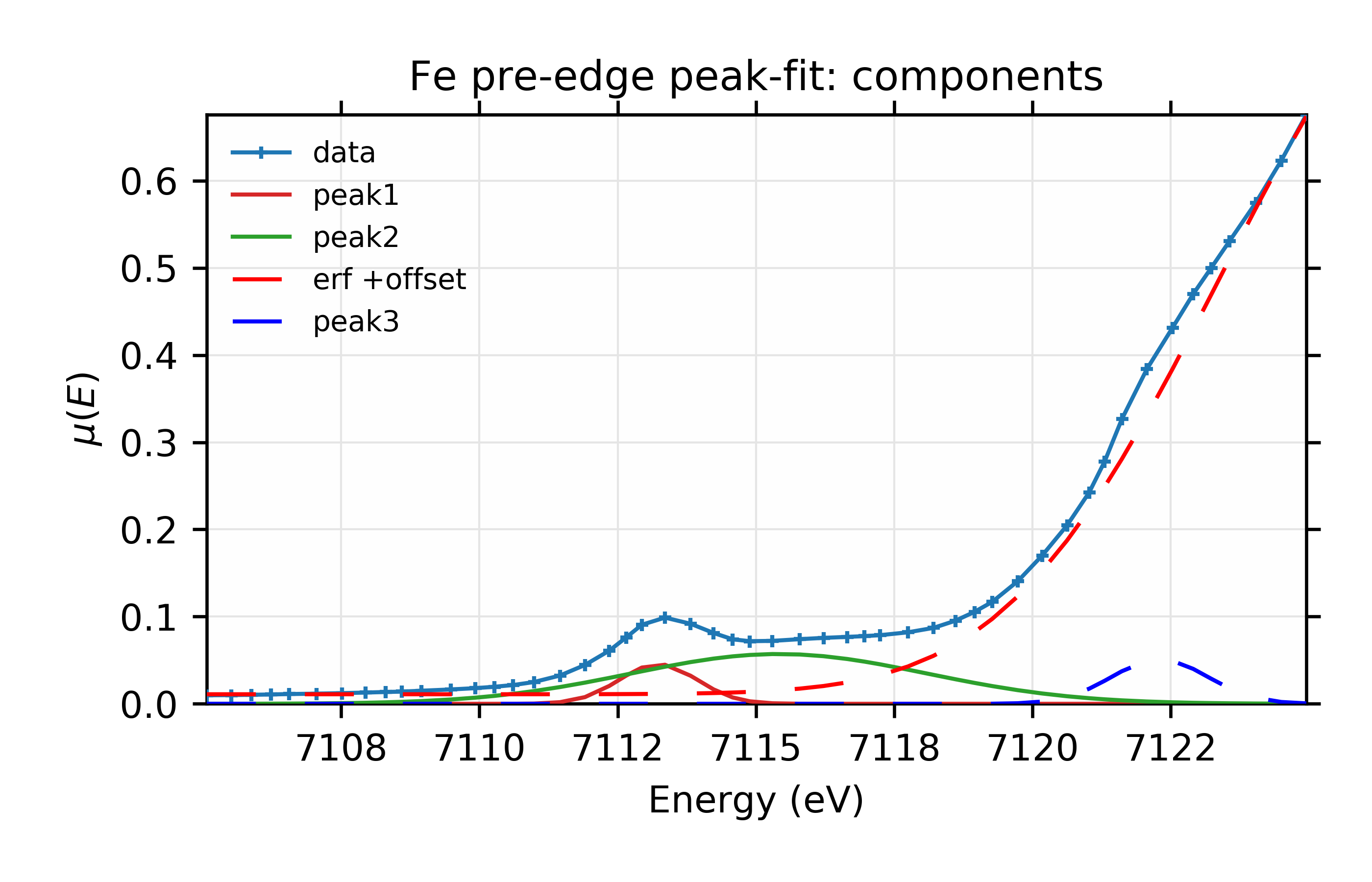
and the plots of the resulting best-fit and components look like these:
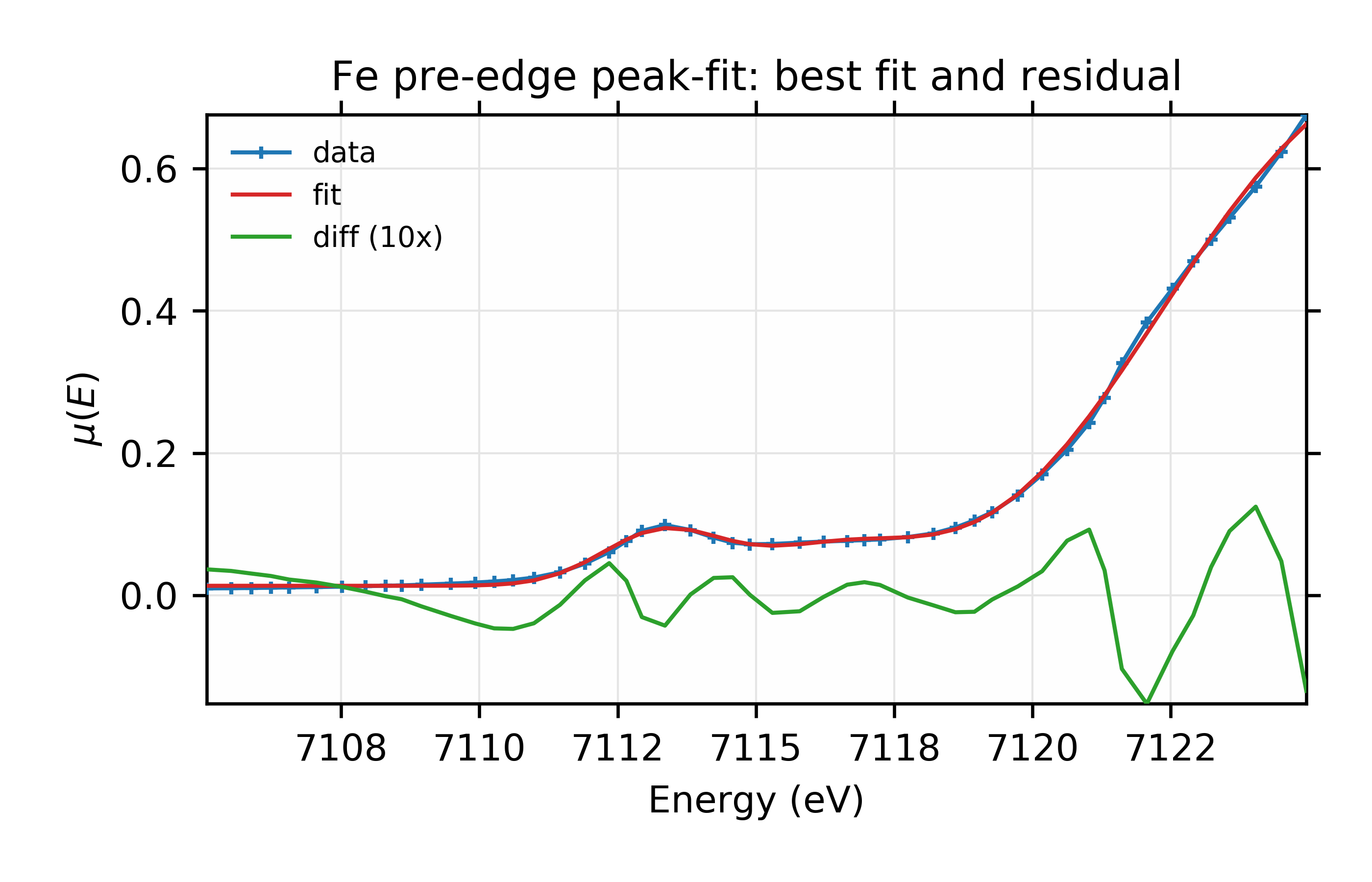 Data, fit, and residual.
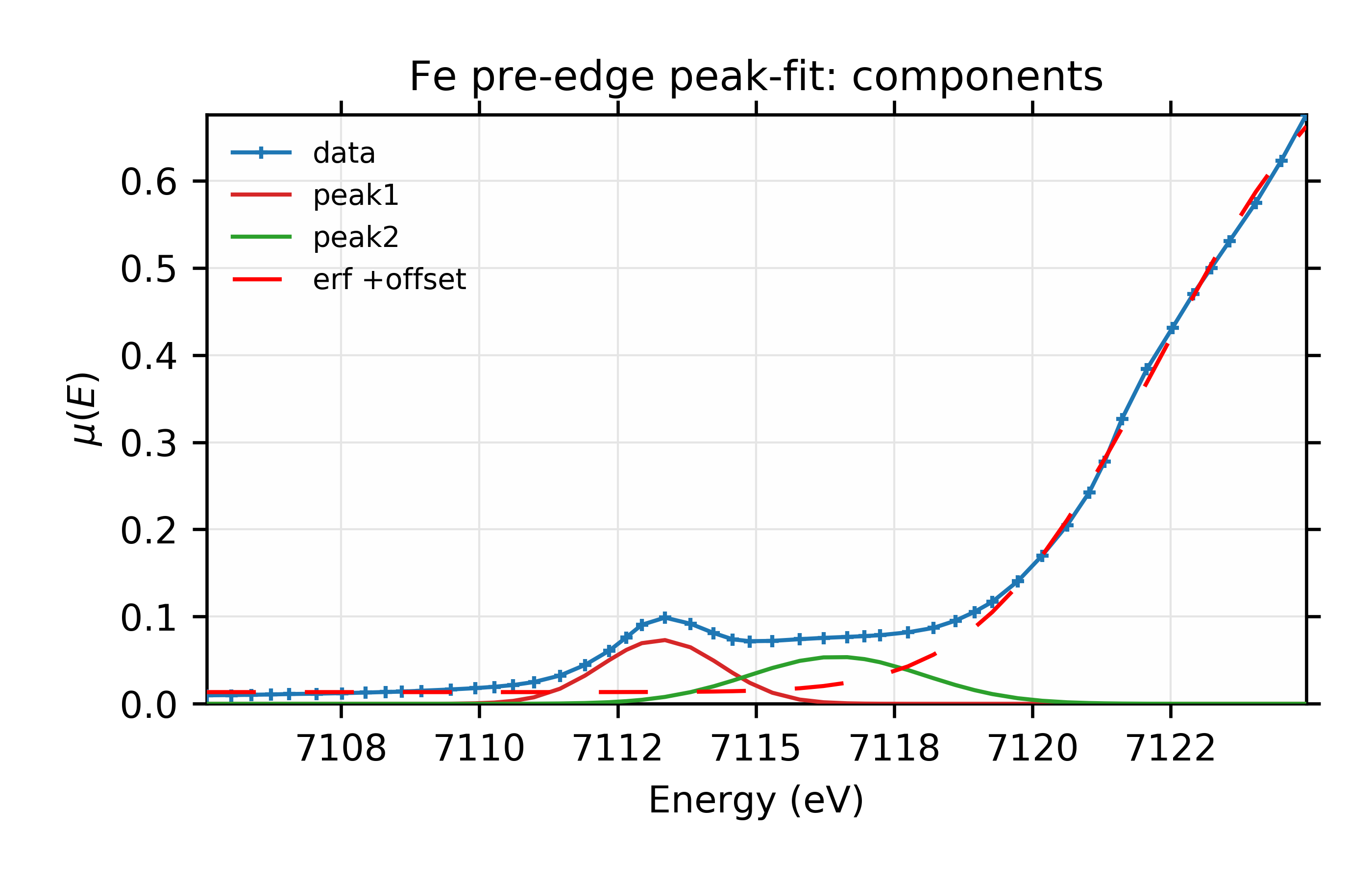 Fit and individual components.
Figure 13.6.2.1 Fit to Fe K-edge pre-edge and edge with 2 Gaussian functions
and we see the fit is pretty good.
Looking more closely, however, there is a hint in the data and the residual
that we may have missed a third peak at around E = 7122 eV. We can add
this by simply adding another peak function to the make_models()
function:
def make_model(pars, data, components=False):
    """make model of spectra: 3 peak functions, 1 erf function, offset"""
    p1 = gaussian(data.e, pars.amp1, pars.cen1, pars.wid1)
    p2 = gaussian(data.e, pars.amp2, pars.cen2, pars.wid2)
    p3 = gaussian(data.e, pars.amp3, pars.cen3, pars.wid3)

    e1 = pars.off + pars.erf_amp * erf( pars.erf_wid*(data.e - pars.erf_cen))
    sum = p1 + p2 + p3 + e1
    if components:
        return sum, p1, p2, p3, e1
    endif
    return sum
enddef
and 3 more fitting parameters to the parameter group:
params = param_group(
    ...
    cen3 = param(7122.0, vary=True, min=7120, max=7124),
    amp3 = param(0.5,    vary=True, min=0),
    wid3 = param(1.2,    vary=True, min=0.05),
    ...)
The fit now has 13 variables, and gives a report like this:
[[Fit Statistics]]
    # function evals   = 504
    # data points      = 51
    # variables        = 13
    chi-square         = 0.00010278
    reduced chi-square = 2.7046e-06
    Akaike info crit   = -642.85
    Bayesian info crit = -617.74
[[Variables]]
    amp1:      0.08005336 +/- 0.005009 (6.26%) (init= 0.25)
    amp2:      0.38406912 +/- 0.017093 (4.45%) (init= 0.25)
    amp3:      0.11105163 +/- 0.016357 (14.73%) (init= 0.5)
    cen1:      7113.23457 +/- 0.023040 (0.00%) (init= 7113.25)
    cen2:      7115.41657 +/- 0.136728 (0.00%) (init= 7116)
    cen3:      7122.30049 +/- 0.039190 (0.00%) (init= 7122)
    erf_amp:   0.47613623 +/- 0.022176 (4.66%) (init= 0.5)
    erf_cen:   7123.37448 +/- 0.215089 (0.00%) (init= 7123.5)
    erf_wid:   0.23023512 +/- 0.009484 (4.12%) (init= 0.5)
    off:       0.48707800 +/- 0.022211 (4.56%) (init= 0.5)
    wid1:      0.70260153 +/- 0.030309 (4.31%) (init= 0.6)
    wid2:      2.68190137 +/- 0.091739 (3.42%) (init= 1.2)
    wid3:      0.86847656 +/- 0.056876 (6.55%) (init= 1.2)
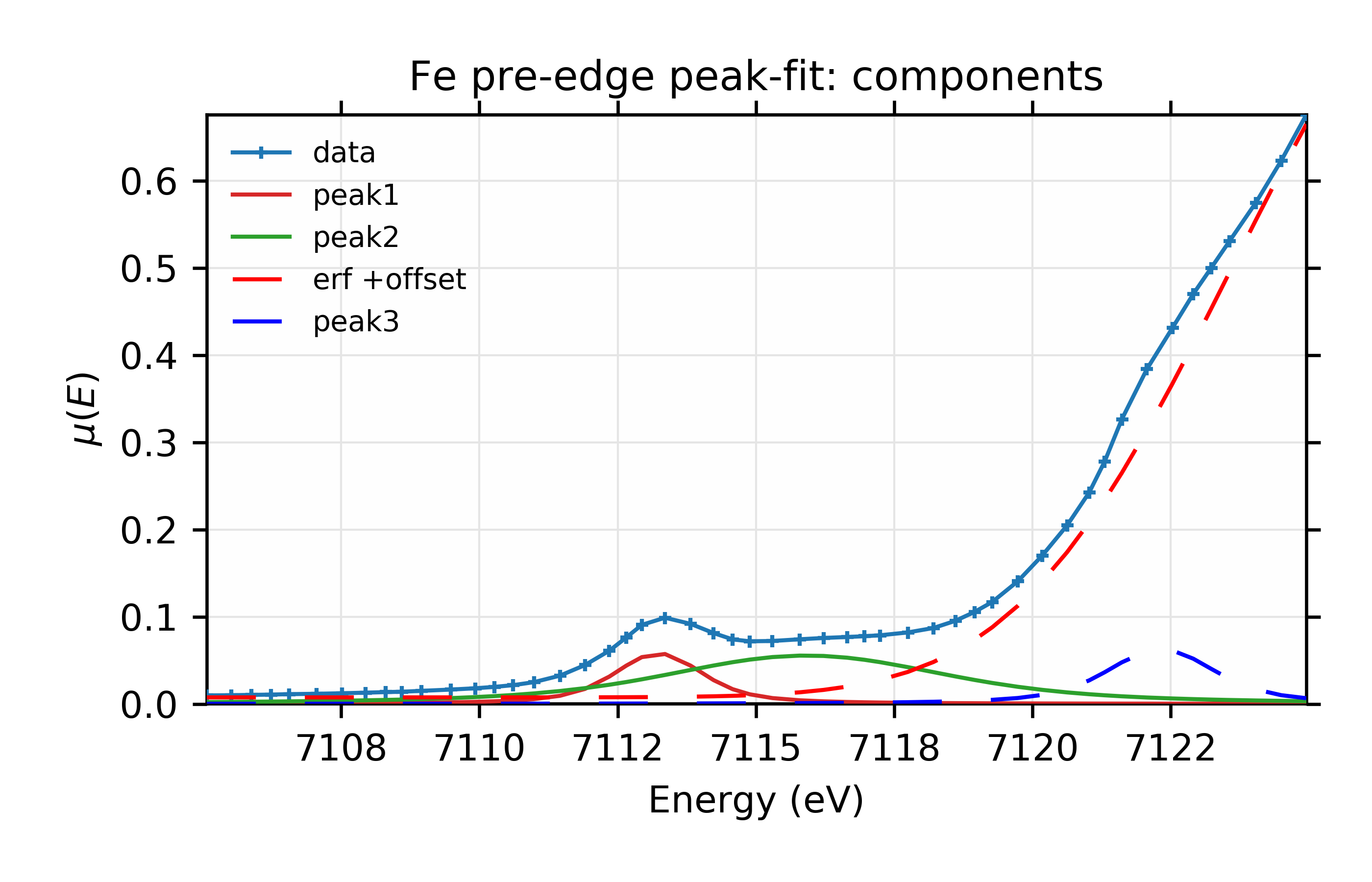
Adding the third peak here reduced \(\chi^2\) by a factor of 10, from 0.001276 to 0.000103, and so seems to be a significant improvement. Reduced chi-square also dropped by an order of magnitude and both the Akaike and Bayesian information criteria dropped by more than 100. The values for the energy center and amplitude for the error function have both moved significantly, as can be seen in the plots for this fit:
 Data, fit, and residual.
 Fit with individual components.
Figure 13.6.2.2 Fit to Fe K-edge pre-edge and edge with 3 Gaussian functions and an Error function.
Finally for this example, we can replace the Gaussian peak shapes with
other functional forms. To use the Voigt function shown in the previous
section, we simply change make_models() to use:
p1 = pars.amp1 * voigt(data.e, pars.cen1, pars.wid1)
p2 = pars.amp2 * voigt(data.e, pars.cen2, pars.wid2)
p3 = pars.amp3 * voigt(data.e, pars.cen3, pars.wid3)
The fit report now reads:
[[Fit Statistics]]
    # function evals   = 476
    # data points      = 51
    # variables        = 13
    chi-square         = 9.2875e-05
    reduced chi-square = 2.4441e-06
    Akaike info crit   = -648.02
    Bayesian info crit = -622.91
[[Variables]]
    amp1:      0.14657959 +/- 0.012760 (8.71%) (init= 0.25)
    amp2:      0.44536523 +/- 0.035916 (8.06%) (init= 0.25)
    amp3:      0.19354556 +/- 0.032364 (16.72%) (init= 0.5)
    cen1:      7113.23780 +/- 0.020989 (0.00%) (init= 7113.25)
    cen2:      7115.91312 +/- 0.134712 (0.00%) (init= 7116)
    cen3:      7122.32066 +/- 0.037577 (0.00%) (init= 7122)
    erf_amp:   0.48986689 +/- 0.023086 (4.71%) (init= 0.5)
    erf_cen:   7123.58055 +/- 0.227490 (0.00%) (init= 7123.5)
    erf_wid:   0.22831037 +/- 0.008305 (3.64%) (init= 0.5)
    off:       0.49735544 +/- 0.023143 (4.65%) (init= 0.5)
    wid1:      0.52826663 +/- 0.027231 (5.15%) (init= 0.6)
    wid2:      1.67565399 +/- 0.093190 (5.56%) (init= 1.2)
    wid3:      0.64297551 +/- 0.047200 (7.34%) (init= 1.2)
and we see that the already very low \(\chi^2\) reduces by another 10%, and improvements of the two information criteria. which suggests a real improvement. For completeness, the plots from this fit look like this:
 Data, fit, and residual.
 Fit with individual components.
Figure 13.6.2.3 Fit to Fe K-edge pre-edge and edge with 3 Voigt functions and an Error function.
It’s difficult to see a dramatic difference in fit quality for this data, but the ability to explore fitting with different lineshapes like this is still a useful test of the robustness of the fit.
13.6.3. Example 3: Fitting XANES Spectra as a Linear Combination of Other Spectra
This example is quite a bit simpler than the previous one, though worth an explicit example. Here, we fit a XANES spectra as a linear combination of two other spectra. This approach is often used to compare an unknown spectra with a large selection of candidate model spectra, taking the result with lowest misfit statistics as the most likely results. Though this method should be used with some caution, it is a standard and very simple approach to XANES analysis.
The example here is borrowed from Bruce Ravel’s data and tutorials, and based on the work published by [Lengke et al. (2006)], The goal here is not to repeat the whole of that analysis, but to present the mechanics of the fitting approach. Essentially, we’re asserting that a particular measured spectrum is made of a linear combination of 2 or more other spectra. We have a set of candidate model spectra, and we’re going to try to determine both which of those model spectra combine to match the measured one. Here we will simply assert that all the spectra are aligned in the ordinate and that they are normalized in some reproducible way so that there are essentially no artefacts or systematic problems in the ‘x’ or ‘y’ values of the data.
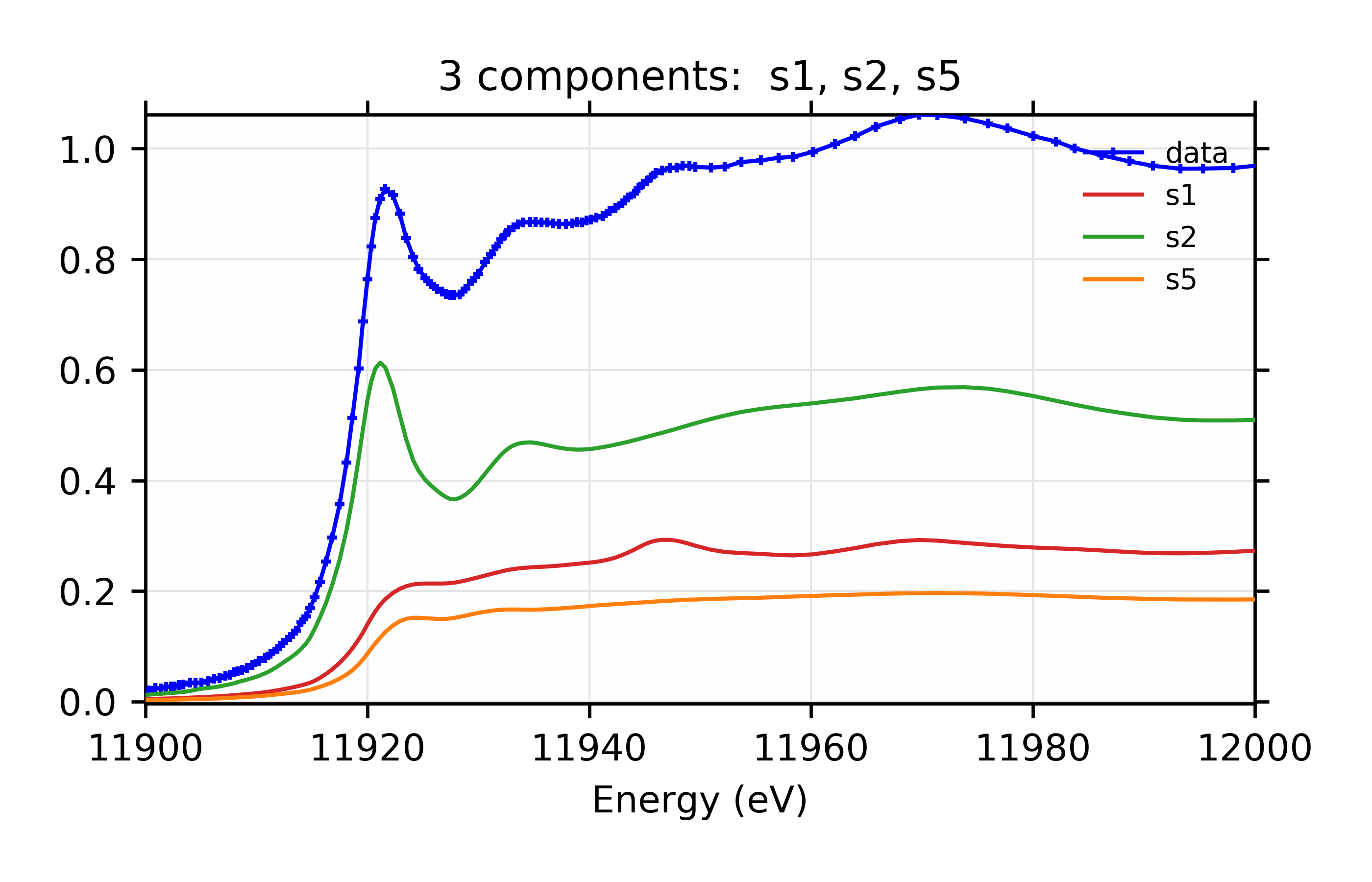
For the example here, the spectra are held in individual ASCII data files, which we’ll call unknown.dat for the unknown spectrum and s1.dat, s2.dat, …, s6.dat for the spectra on 6 different standards. It is not important for the discussion here what these spectra represent, but they are XANES data taken at the Au L3 edge on various Au compounds.
A visual inspection of the spectra (see Figure 13.6.3.1) suggests that s2 is probably a major component of the unknown, though the peak around 11950 eV is a feature that only s1 has, so it too may be an important component.
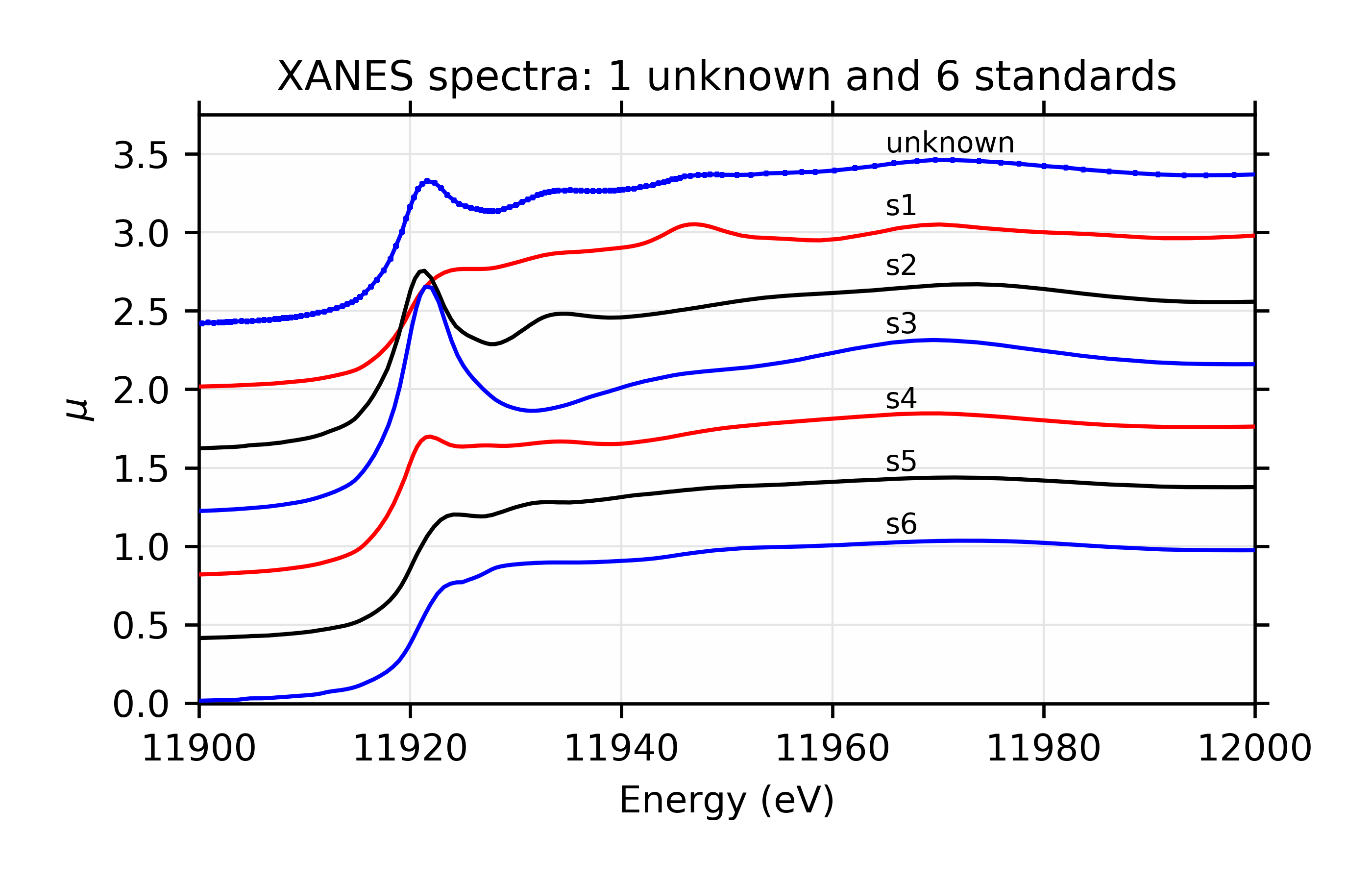 Components used for linear combinations.
 Fit and residual with components *s1* and *s2*.
Figure 13.6.3.1 Linear Combination Fit of gold XANES in cyanobacteria, after [Lengke et al. (2006)].
To quantitatively fit these spectra, we read in all the data, and then create a single group dat that will contain all the data we need. It turns out (and a common issue for XAFS data), the scans here do not have identical energy values, so we both select a limited energy range, and interpolate the standards onto the energy array of the unknown, and put all these spectra into a single group:
## examples/fitting/doc_example3/ReadData.lar
d1 = read_ascii('unknown.dat')
s1 = read_ascii('s1.dat')
s2 = read_ascii('s2.dat')
s3 = read_ascii('s3.dat')
s4 = read_ascii('s4.dat')
s5 = read_ascii('s5.dat')
s6 = read_ascii('s6.dat')

i1, i2 = index_of(d1.energy, 11870), index_of(d1.energy, 12030)

data = group(energy=d1.energy[i1:i2+1], mu=d1.munorm[i1:i2+1])

data.s1 = interp(s1.energy, s1.munorm, data.energy)
data.s2 = interp(s2.energy, s2.munorm, data.energy)
data.s3 = interp(s3.energy, s3.munorm, data.energy)
data.s4 = interp(s4.energy, s4.munorm, data.energy)
data.s5 = interp(s5.energy, s5.munorm, data.energy)
data.s6 = interp(s6.energy, s6.munorm, data.energy)
## end of examples/fitting/doc_example3/ReadData.lar
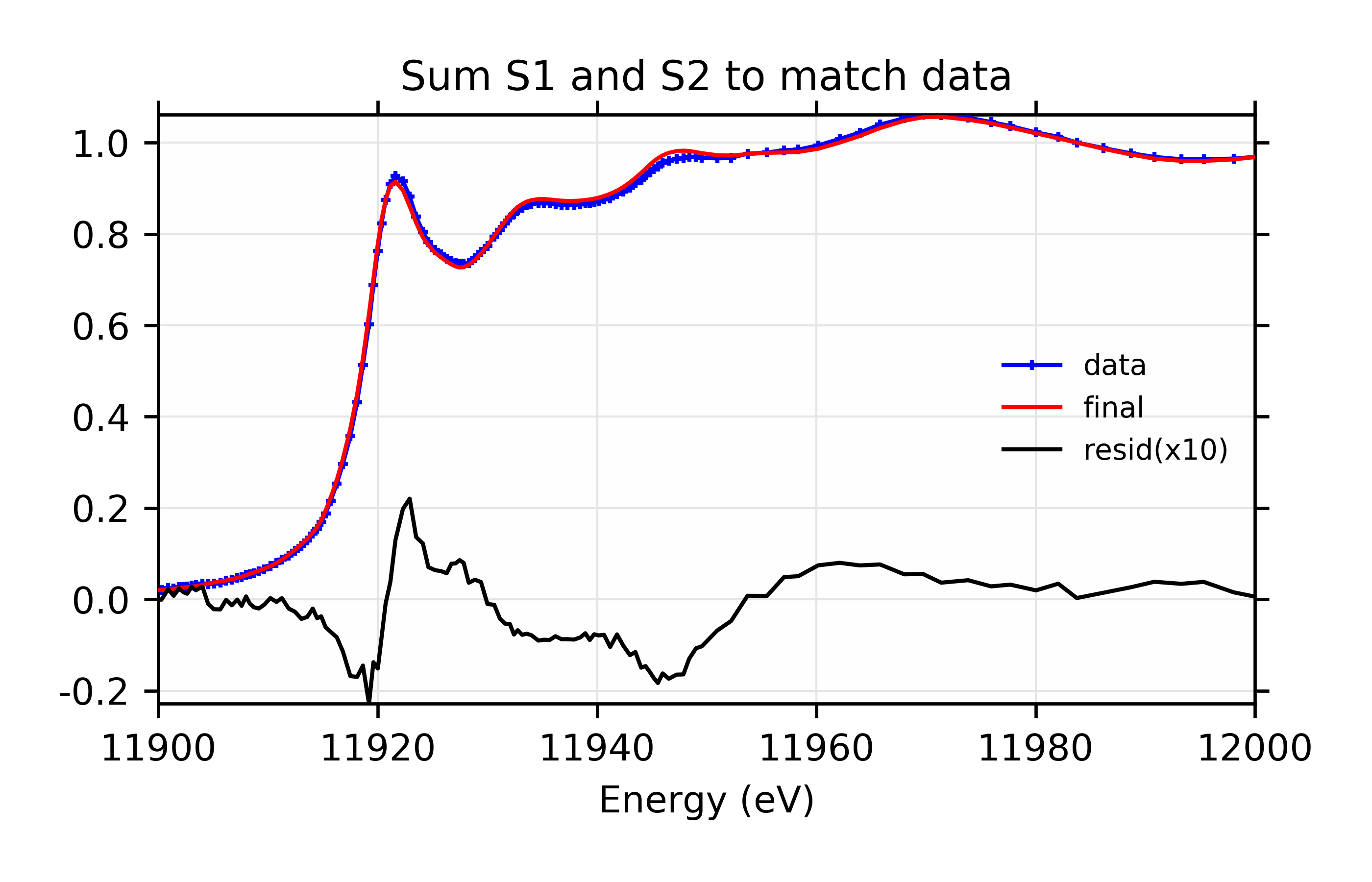
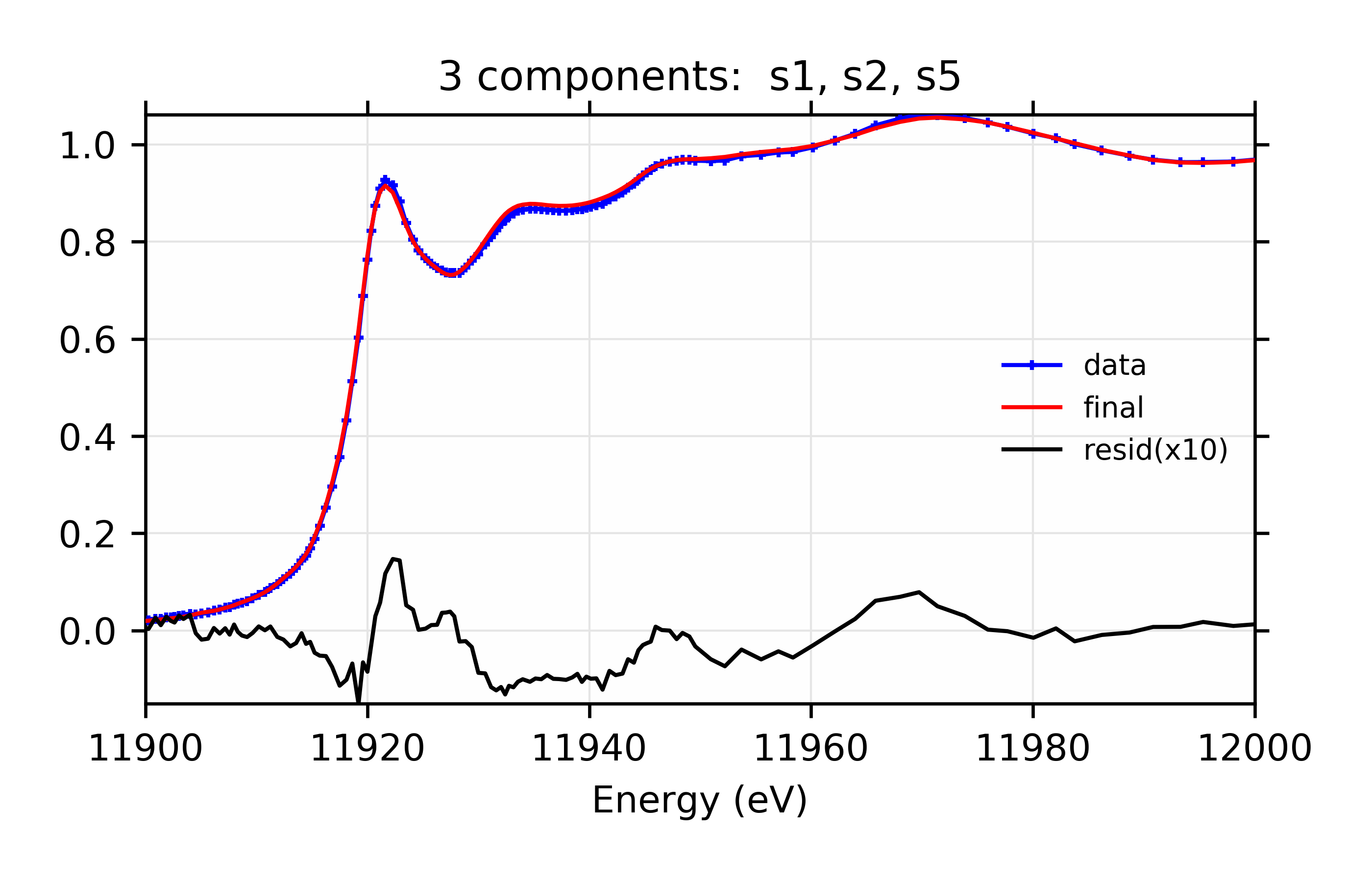
The initial fit to the unknown spectrum with spectra s1 and s2 looks like this:
## examples/fitting/doc_example3/fit1.lar
run('ReadData.lar')


# create a parameter group for the fit:
params = group(amp1 = param(0.5, min=0, max=1),
               amp2 = param(0.5, min=0, max=1),
               amp3 = param(0.0, min=0, max=1),
               amp4 = param(0.0, min=0, max=1),
               amp5 = param(0.0, min=0, max=1),
               amp6 = param(0.0, min=0, max=1))

# define objective function for fit residual
def sum_standards(pars, data):
    return (pars.amp1*data.s1 + pars.amp2*data.s2 + pars.amp3*data.s3 +
            pars.amp4*data.s4 + pars.amp5*data.s5 + pars.amp6*data.s6 )
#enddef

def resid(pars, data):
    return (data.mu - sum_standards(pars, data))/data.eps
#enddef

# set model here: Amp1 is free,
# Amp2 is constrained to be 1 - Amp1

params.amp1.vary = True
params.amp2.expr = '1 - amp1'

# set uncertainty in data that we'll use to scale the returned residual
data.eps  = 0.001

# perform fit
result = minimize(resid, params, args=(data,))
fit = sum_standards(params, data)
print fit_report(result)


plot(data.energy, data.mu,   label='data', color='blue', marker='+',
     markersize=5, show_legend=True, legend_loc='cr', new=True,
     xlabel='Energy (eV)', title='Sum S1 and S2 to match data',
     xmin=11900, xmax=12000)
plot(data.energy, fit,  label='final', color='red')

plot(data.energy, 10*(data.mu-fit),  label='resid(x10)', color='black')

## end of examples/fitting/doc_example3/fit1.lar
Here, we actually define a weight for all 6 spectra, but force 4 of them to
be 0. For a two component fit, this would not be necessary, but we’ll be
expanding this shortly. We place bounds of [0, 1] on all the parameters,
and we use a constraint to ensure that the parameters add to 1.0. Also
note that we define an uncertainty in the data that we use to scale the
data - model returned by the fit. This is somewhat arbitrarily chosen
to be 0.001, that is 0.1% of the typical data value. The
results of this fit are:
[[Fit Statistics]]
    # function evals   = 7
    # data points      = 160
    # variables        = 1
    chi-square         = 9339.1
    reduced chi-square = 58.736
    Akaike info crit   = 652.69
    Bayesian info crit = 655.76
[[Variables]]
    amp1:   0.47066003 +/- 0.004708 (1.00%) (init= 0.5)
    amp2:   0.52933996 +/- 0.004708 (0.89%)  == '1 - amp1'
    amp3:   0 (fixed)
    amp4:   0 (fixed)
    amp5:   0 (fixed)
    amp6:   0 (fixed)
and the result for this fit is shown in Figure 13.6.3.1. This demonstrates the use of simple constraints for Parameters in fits: we’ve used an algebraic expression to ensure that the weights for the two components in the fit add to 1.
The fit here is not perfect, and we suspect there may be another standard as a component to the fit. But at this point, we have several candidate spectra, and a pretty good starting fit, so the main questions are
How do we know when one fit is better than another?
Which combination gives the best results?
To answer the first question, we’ll assert that “improved reduced chi-square” is the best way to decide which of a series of fits is best. To answer the second question, we’ll work through all the possibilities. Now, we set up a more complicated script to do 5 separate fits so that we can compare the results. This makes use of some of the more advanced scripting features of larch:
## examples/fitting/doc_example3/fit2.lar
run('ReadData.lar')

# define objective function for fit residual
def sum_standards(p, data):
    return (p.amp1*data.s1 + p.amp2*data.s2 + p.amp3*data.s3 +
            p.amp4*data.s4 + p.amp5*data.s5 + p.amp6*data.s6 )
enddef

def resid(pars, data):
    """residual function for minimization"""
    out = data.mu - sum_standards(pars, data)
    if hasattr(data, 'eps'):
        out = out / data.eps
    endif
    return out
enddef

params = param_group(amp1 = param(0.4, vary=True, min=0, max=1),
                     amp2 = param(0.4, vary=True, min=0, max=1),
                     amp3 = param(0.0, min=0, max=1),
                     amp4 = param(0.0, min=0, max=1),
                     amp5 = param(0.0, min=0, max=1),
                     amp6 = param(0.0, min=0, max=1),  note = '')

# make 4 copies of this parameter group:
pars = []

# Model:  two components only (same as fit1)
pars.append(copy(params))
pars[0].amp2.vary = False
pars[0].amp2.expr = '1 - amp1'
pars[0].note = '2 components:  s1, s2'

# Model: three components
pars.append(copy(params))
pars[1].amp3.expr = '1 - amp1 - amp2'
pars[1].note = '3 components:  s1, s2, s3'

# Model: three components
pars.append(copy(params))
pars[2].amp4.expr = '1 - amp1 - amp2'
pars[2].note = '3 components:  s1, s2, s4'

# Model: three components
pars.append(copy(params))
pars[3].amp5.expr = '1 - amp1 - amp2'
pars[3].note = '3 components:  s1, s2, s5'

# Model: three components
pars.append(copy(params))
pars[4].amp6.expr = '1 - amp1 - amp2'
pars[4].note = '3 components:  s1, s2, s6'

# set uncertainty in data that we'll use to scale the returned residual
data.eps  = 0.001


## Now loop over parameter groups, performing fit and comparing
## the value of reduced chi-square, AIC and BIC
print 'chi_reduced |  A I C  |  B I C | Notes'
print '------------+---------+--------+----------------------------'
best_chi2, best_params = 1.e99, None
fmt = ' %8.1f   | %6.1f  | %6.1f |  %s'
for p in pars:
    ret = minimize(resid, p, args=(data,))
    print fmt % (ret.chi_reduced, ret.aic, ret.bic, p.note)
    if ret.chi_reduced < best_chi2:
        best_params, best_result, best_chi2 = p, ret, ret.chi_reduced
    #endif
#endfor
print '------------+---------+--------+----------------------------'


def make_plots(pars, d):
    "generates best-fit plots for a parameter group"
   fit = sum_standards(pars, d)
   plot(d.energy, d.mu,   label='data', color='blue', marker='+',
        markersize=5, show_legend=True, legend_loc='cr', new=True,
        xlabel='Energy (eV)', title=pars.note, xmin=11900, xmax=12000)
   plot(d.energy, fit,  label='final', color='red')
   plot(d.energy, 10*(d.mu-fit),  label='resid(x10)', color='black')

   # window 2: components
   plot(d.energy, d.mu,  label='data', color='blue', marker='+',
        markersize=5, show_legend=True, legend_loc='ur', new=True, win=2,
        xlabel='Energy (eV)', title=pars.note, xmin=11900, xmax=12000)
   if pars.amp1 != 0:  plot(d.energy, pars.amp1*d.s1, label='s1', win=2)
   if pars.amp2 != 0:  plot(d.energy, pars.amp2*d.s2, label='s2', win=2)
   if pars.amp3 != 0:  plot(d.energy, pars.amp3*d.s3, label='s3', win=2)
   if pars.amp4 != 0:  plot(d.energy, pars.amp4*d.s4, label='s4', win=2)
   if pars.amp5 != 0:  plot(d.energy, pars.amp5*d.s5, label='s5', win=2)
   if pars.amp6 != 0:  plot(d.energy, pars.amp6*d.s6, label='s6', win=2)
enddef

print 'Best Fit:  ', best_params.note
# NOTE!  set paramGroup to best_params to ensure
#        that constraintes are properly evaluated

print fit_report(best_result)

make_plots(best_params, data)

## end of examples/fitting/doc_example3/fit2.lar
There are several points worth noting here:
We make a new copy of the Parameter Group for each fit – this way we can (with some care) switch back and forth between fitting models. Note that we add the non-Parameter
notemember to this group that give a brief description of the fit. Of course, we could add anything else we wanted.We set
amp1.varyandamp2.varytoTrueand set one of the other amplitude parameter’s expression to1 - amp1 - amp2to impose the desired constraint.The loop over Parameter groups runs the fit for each set of Parameters, and checks for the lowest value of
chi_reduced,aic, andbic.
The output of running this gives:
chi_reduced |  A I C  |  B I C | Notes
------------+---------+--------+----------------------------
     58.7   |  652.7  |  655.8 |  2 components:  s1, s2
     40.2   |  592.9  |  599.1 |  3 components:  s1, s2, s3
     37.2   |  580.6  |  586.7 |  3 components:  s1, s2, s4
     32.1   |  557.2  |  563.4 |  3 components:  s1, s2, s5
     37.2   |  580.6  |  586.8 |  3 components:  s1, s2, s6
------------+---------+--------+----------------------------
Best Fit:   3 components:  s1, s2, s5
[[Fit Statistics]]
    # function evals   = 12
    # data points      = 160
    # variables        = 2
    chi-square         = 5078.3
    reduced chi-square = 32.141
    Akaike info crit   = 557.21
    Bayesian info crit = 563.36
[[Variables]]
    amp1:   0.27866516 +/- 0.017035 (6.11%) (init= 0.4)
    amp2:   0.53207041 +/- 0.003491 (0.66%) (init= 0.4)
    amp3:   0 (fixed)
    amp4:   0 (fixed)
    amp5:   0.18926442 +/- 0.016438 (8.69%)  == '1 - amp1 - amp2'
    amp6:   0 (fixed)
[[Correlations]] (unreported correlations are <  0.100)
    C(amp1, amp2)                = -0.270
and the output plots for the best model look like this:
 Linear combination fit and residual.
 Weighted contribution from individual components.
Figure 13.6.3.2 Linear Combination XANES Fit of gold components in cyanobacteria with species s1, s2, and s5.
Of course, we aren’t necessarily done here as we haven’t exhausted all possible combinations of components. Included in the examples (examples/fitting/doc_examples3/fit3.lar), but not reprinted here, is a script that runs through all possible combinations of 3 and 4 components, though still assuming that s1 and s2 are components.
The output gives this:
chi_reduced | A I C | B I C | Notes
------------+---------+--------+----------------------------
58.7 | 652.7 | 655.8 | 2 component fit: s1, s2
40.2 | 592.9 | 599.1 | 3 component fit: s1, s2, s3
37.2 | 580.6 | 586.7 | 3 component fit: s1, s2, s4
32.1 | 557.2 | 563.4 | 3 component fit: s1, s2, s5
37.2 | 580.6 | 586.8 | 3 component fit: s1, s2, s6
59.2 | 656.0 | 665.2 | 4 component fit: s1, s2, s3, s4
14.7 | 433.3 | 442.5 | 4 component fit: s1, s2, s3, s5
13.3 | 417.6 | 426.8 | 4 component fit: s1, s2, s3, s6
30.1 | 547.8 | 557.1 | 4 component fit: s1, s2, s4, s5
32.4 | 559.2 | 568.5 | 4 component fit: s1, s2, s5, s6
34.3 | 568.8 | 578.0 | 4 component fit: s1, s2, s4, s6
------------+---------+--------+----------------------------
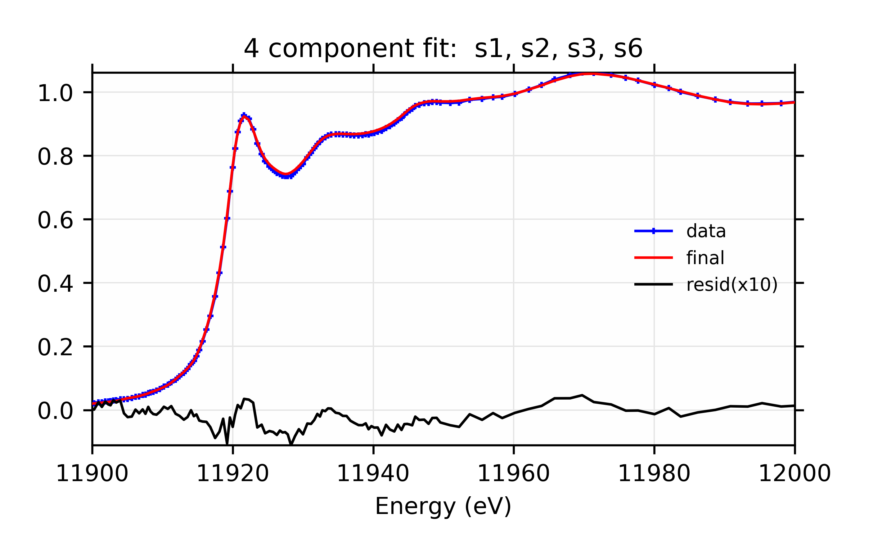
Best Fit: 4 component fit: s1, s2, s3, s6
[[Fit Statistics]]
# function evals = 37
# data points = 160
# variables = 3
chi-square = 2095.2
reduced chi-square = 13.345
Akaike info crit = 417.56
Bayesian info crit = 426.78
[[Variables]]
amp1: 0.32788267 +/- 0.009491 (2.89%) (init= 0.4)
amp2: 0.46501286 +/- 0.005624 (1.21%) (init= 0.4)
amp3: 0.06384062 +/- 0.003749 (5.87%) (init= 0)
amp4: 0 (fixed)
amp5: 0 (fixed)
amp6: 0.14326383 +/- 0.008029 (5.60%) == '1 - amp1 - amp2 - amp3'
[[Correlations]] (unreported correlations are < 0.100)
C(amp2, amp3) = -0.890
C(amp1, amp2) = -0.340
You might notice that, whereas the 3 component fit favored adding s5, the four component fit favors s3 and s6. You might further notice that the four component fit with s3 and s5 has reduced chi-square of 14.7, only slightly worse than the best value. For completeness, the parameters for that are:
larch> ret6 = minimize(resid, pars[6], args=(data,))
larch> print fit_report(ret6)

[[Fit Statistics]]
    # function evals   = 7
    # data points      = 160
    # variables        = 3
    chi-square         = 2312.1
    reduced chi-square = 14.727
    Akaike info crit   = 433.32
    Bayesian info crit = 442.55
[[Variables]]
    amp1:   0.30304286 +/- 0.011667 (3.85%) (init= 0.3030429)
    amp2:   0.45835749 +/- 0.005874 (1.28%) (init= 0.4583575)
    amp3:   0.05429199 +/- 0.003961 (7.30%) (init= 0.05429198)
    amp4:   0 (fixed)
    amp5:   0.18430763 +/- 0.011132 (6.04%)  == '1 - amp1 - amp2 - amp3'
    amp6:   0 (fixed)
[[Correlations]] (unreported correlations are <  0.100)
    C(amp2, amp3)                = -0.916
    C(amp1, amp2)                = -0.247
    C(amp1, amp3)                =  0.152
The plots resulting from both sets of Parameters are shown:
 Data, fit, and residual.
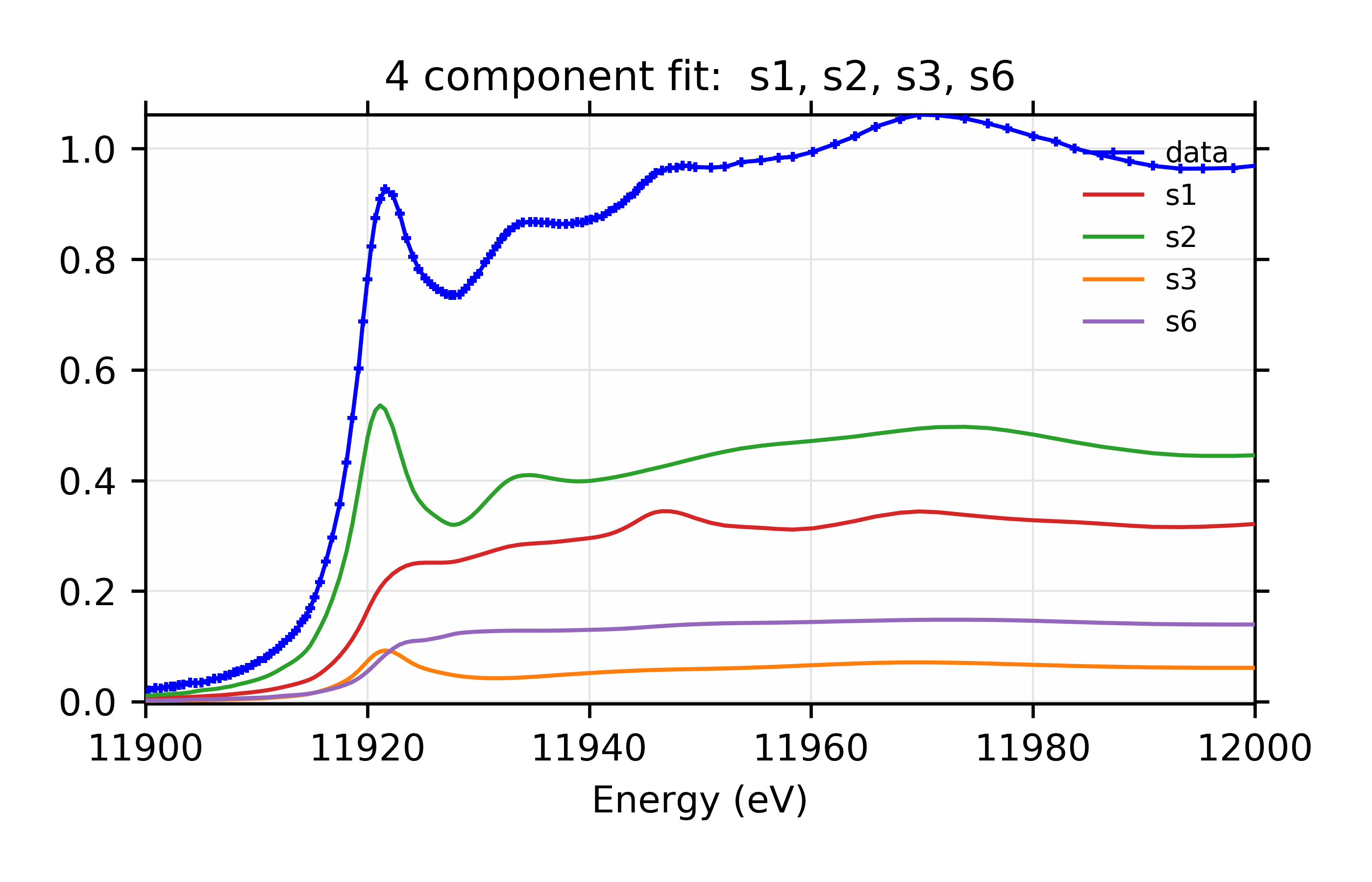 Weighted contribution from individual components.
Figure 13.6.3.3 Linear Combination XANES Fit of gold components in cyanobacteria with species s1, s2, s3, and s6.
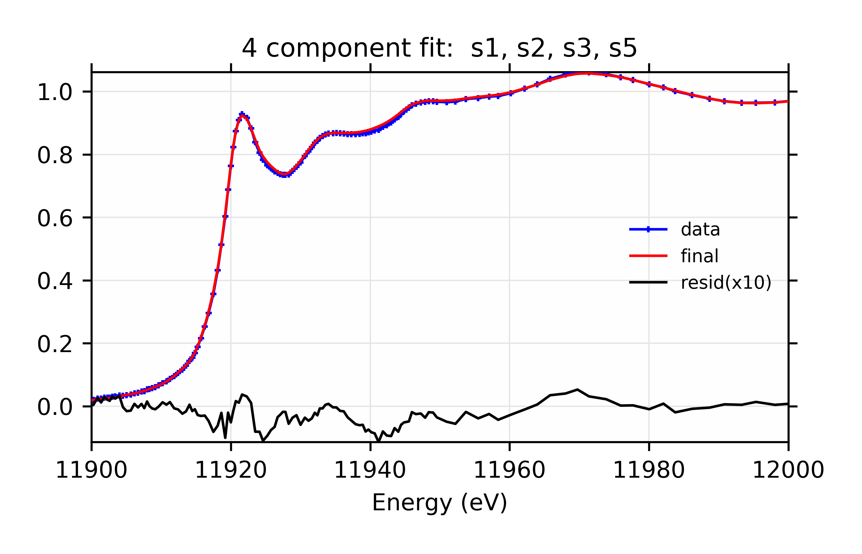 Linear Combination XANES Fit of gold components in
cyanobacteria with species *s1*, *s2*, *s3*, and
*s5*. Data, fit, and residual.
Linear Combination XANES Fit of gold components in
cyanobacteria with species *s1*, *s2*, *s3*, and
*s5*. Data, fit, and residual.
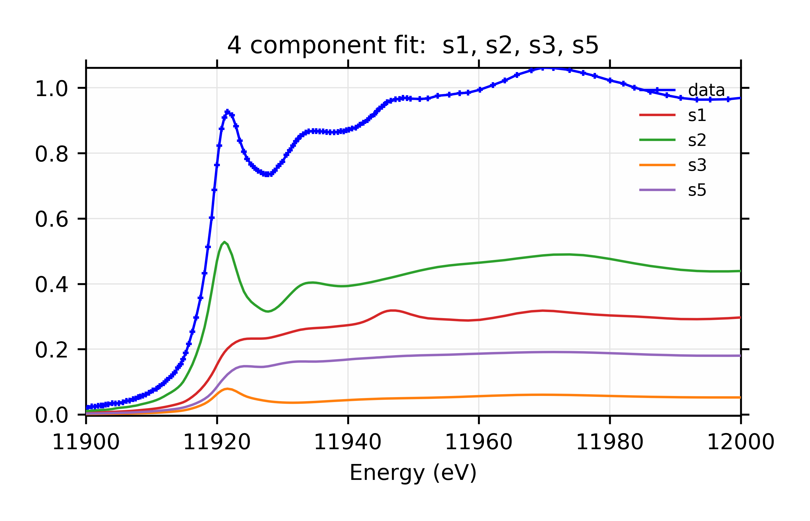 Weighted contribution from individual components.
Figure 13.6.3.4 Linear Combination XANES Fit of gold components in cyanobacteria with species s1, s2, s3, and s5.
From the plots alone, it is difficult to tell which of these fits is better, and it is probably best to say that these are both good fits. This implies that component s3 is important even if at a very small fraction, and that either component s5 or s6 (which aren’t that different spectroscopically or chemically (see Figure 13.6.3.1) is present. Of course, the analysis here is not meant to be definitive, and there are many more checks that could be done. To be clear, [Lengke et al. (2006)] looked at many more unknown spectra, and also adjusted the energy ranges of the fits, and concludedd that s1, s2, s3, and s5 were the best components, with concentrations of the components very similar to the ones found here.