\(\newcommand{\AA}{\unicode{x212B}}\)
5.1. Larix Overview
Larix is Graphical User Interface program for working with X-ray Absorption Spectroscopy (XAS) data. The program is intended to be useful for both novices and experts of XAS, and the aim is to include all analytic methods used for XAS data. While the program emphasizes rapid and interactive data visualization and analysis, analysis can generally be applied to multiple spectra. In addition, all analysis steps are recorded in a way that is readily converted to a Python program or script for reproducible and batch processing of large numbers of spectra. Two of the most important concepts for using XAS Viewer are:
Larix organizes all XAS Spectra into Groups of data. In fact, the words “Spectra” and “Group” may be used interchangeably here. For each spectrum, the raw data, any processed data arrays, all settings, and even fitting results will be contained in a single Group, separate from all other spectra.
To the extent possible, all data processing and analysis steps, and even most of the visualization steps in Larix will be done in the Larch interpreter and shown in the Larch Buffer (Basic Larch GUI) as they are executed. This not only displays the steps taken, but records them in as high-level Python code that can be saved and used to create batch processing scripts and to give reproducible analyses. If, at any point you want to know exactly what Larix is “really doing”, you can open the Larch Buffer and see the commands being executed.
With those overall goals in mind, the main features of Larix can be broken into a few categories. Here we give a brief overview, and then expand on these topics in the following sections.
5.1.1. Basic Layout, GUI Controls, and XAS Data Management
Each XAS Spectra or Group of data will be displayed in a list of Spectra of the main Larix window. This list will show the “File Name” for each spectra/group which will usually be derived from the name of the file from which the data was read. Since a data files might give multiple spectra and since some Groups of data will be generated by Larix, the list here really gives a unique name for each group that will be used to identify it throughout Larix.
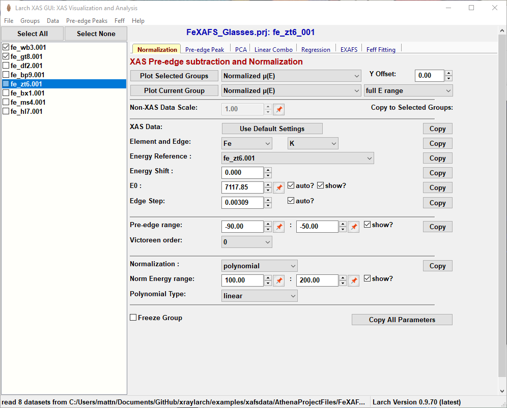
Figure 5.1.1.1 Larix showing the File/Group list on the left-hand side and the set of Working Panels in a “Tabbed Display” on the left-hand side for various data processing and analysis tasks. The XAS pre-edge subtraction and normalization panel is shown by default.
5.1.1.1. List of Spectra
Larix opens with a main window as shown in Figure 5.1.1.1, after some data has been read in. The left-hand side contains a list of spectra groups that have been read. Clicking on the file name makes that group of data the “current data group”, while checking the boxes next to each name will select multiple Groups. Buttons at the top of the list of files can be used to “Select All” or “Select None”. Right-clicking (or “Control-Mouse” on macOS) on the file list will pop up a menu that will allow you to copy, remove, or rename a Group, or view the Journal of processing steps for it. From this pop-up window you can also re-order the list or make more fine-scale selections of spectra.
In addition to the displayed File Name, each Group will also have an internal “Group Name”, which is the name of the Python symbol in the Larch interpreter used to access this Group of data. This group name will be automatically generated using the more restrictive limitations on what characters can be used, and so is somewhat less useful for displaying as the name of the group, but will be how this Group of data is accessed in the Larch buffer.
As hinted at above, each Group will also have a Journal associated with it. The journal will contain the history of processing steps done for that group, usually with detailed, human-readable parameters used in the processing. When saving and loading Session files, these Journals are preserved across data analysis sessions.
5.1.1.2. Notebook Tabs
While the List of Spectra is shown on the left-hand side of the Larix window, the right-hand side shown in Figure 5.1.1.1 contains multiple forms or “Work Panels” for various data processing and analysis tasks that are arranged in a tabbed notebook display. On startup, the work panel labelled “Normalization” is shown for for pre-edge subtraction and normalization (for more detail, see Pre-edge subtraction and Normalization). Other notebook tabs include panels for fitting pre-edge peaks (Pre-edge peak fitting), Linear Combination Analysis (Linear Combination Analysis), Principal Component Analysis (Principal Component and Non-negative Factor Analysis), Advanced Linear Regression (Linear Regression with LASSO and PLS to predict external variable), EXAFS Data Processing (EXAFS Processing: Background Subtraction and EXAFS Processing: Fourier Transforms), and Feff fitting (Fitting EXAFS data to Feff Paths). These panels generally assume that data has been pre-edge subtracted and normalized. Each of these will be covered in more detail below.
5.1.1.3. GUI Controls, and using the Pin icon
Most of the GUI controls should be pretty familiar. Several of the fields for numerical values only allow valid numbers. Some of these also have arrows to increment or decrement the value by an appropriate amount for that value.
Several numerical values also have a button with a ‘pin’ icon ![]() just to the
right of the value. This pin button allows you to select a value from the
current plot window. Clicking this button and then clicking anywhere on the
plot window will use the X value (or occasionally the Y value) from the point
selected on the plot to fill in the value for that field. The ‘pin’ icon is
used in many of the work panels of Larix, including the Normalization
panel.
just to the
right of the value. This pin button allows you to select a value from the
current plot window. Clicking this button and then clicking anywhere on the
plot window will use the X value (or occasionally the Y value) from the point
selected on the plot to fill in the value for that field. The ‘pin’ icon is
used in many of the work panels of Larix, including the Normalization
panel.
5.1.1.5. Plotting Window
Interactive data visualization is an important component of Larix. On startup, a plot window will be shown for plotting X/Y line plots, the most common way to plot XAS data. Larix will display many different datasets in this way, all made with Larch (see Plotting and Displaying Data) and wxmplot. These plots are highly interactive, customizable, and can produce publication-quality images. The plots can be zoomed in and out, and can be configured to change the colors, linestyles, margins, text for labels, and more. While Larix starts up with one plot window, some analysis tasks will bring up a second plot window. A few windows for browsing analysis results will even allow you to bring up more and choose which window to plot to.
From any plot window you can use Ctrl-C to copy the image to the clipboard, Ctrl-S to Save the image as PNG file, or Ctrl-P to print the image with your systems printer. Ctrl-K will bring up a window with forms to configure the colors, text, styles and so on. These common options are available from the File and Options menu of the plotting window.
In particular, clicking on the legend for any labeled curve on a plot will toggle whether that curve is displayed and partially lighten the label itself. This feature of the plotting window means that Larix may draw several different traces on the same plot window and allow (or even expect) you to turn some of them on or off interactively to better view the different components being shown. This can be especially useful for comparing XANES spectra or for inspecting the results of peak fitting.
Larix starts up with one plot window. Some analysis tasks will bring up a second plot window, and a few displays of analysis results will allow you to bring up more and choose which window to plot to.
5.1.2. Data Input and Output
Larix can import XAS data in the following formats
XDI data files - the standard data format for XAS data (Reading Plain text data files, including XDI).
plain text data data files with data arrays in column format (Reading Plain text data files, including XDI), including data files from most XAS beamlines at most facilities.
Athena Project Files (Reading Data from Athena Project Files).
ESRF Spec/BLISS HDF5 files (Reading Spec/Bliss HDF5 Data).
Larch Session files (Larch Session Files and Larix).
Plain text files with non-XAS data, such as line-up scans or X-ray emission spectra can also be read in, and some support for plotting is available for them.
For saving and exporting data, Larix can save multiple XAS spectra as:
Athena Project files (Reading Data from Athena Project Files).
CSV files, from selected groups or for fitting and analysis results.
Larch Session files (Larch Session Files and Larix).
See Reading and Saving Data into Larix for details.
5.1.3. Data Normalization
The first task for working with XAS data is to subtract the pre-edge and normalize the data, so that normalized XAFS (which goes from 0 below the absorption edge to 1 above the absorption edge) is available for downstream analysis. The “Normalization” panel of Larix shows most of the parameters needed for selecting the energy threshold value ‘E0’, doing pre-edge subtraction, and estimating the value of the edge step.
This step is also typically where data corrections and summing of multiple spectra will be done. There are variety of Task-specific Dialog boxes may be used to perform optional data processing and analysis tasks. These dialogs are brought up from the Menu of the Larix window, and include tools for the following data processing operations:
Merging Spectra: adding together the \(\mu(E)\) signals.
Rebinning of data onto a different energy grid
Remove glitches or truncating data.
Smoothing of data.
Deconvolution of data.
Correcting for Over-absorption of fluorescence XANES data.
All of these data processing steps can be done interactively for any group of data, and the user is able to adjust a small set of curated parameters and then visualize the results of these adjustments.
5.1.4. XANES Analysis
For XANES analysis, Larix supports the following data analysis processes:
linear combination analysis of spectra.
principal component analysis.
regression of XANES spectra with a predicting external variable.
pre-edge peak fitting.
Each of these is given its own “Tab” in the main Larix window.
5.1.5. EXAFS Processing
For EXAFS analysis, the EXAF XANES analysis, Larix supports the following data analysis processes:
EXAFS background spline removal.
forward Fourier transforms from \(k\) to \(R\)
back Fourier transforms from \(R\) to filtered-\(k\) space
Cauchy wavelet transforms.
5.1.6. EXAFS Modeling with FEFF
Browser for CIF files from American Mineralogist Crystal Structure Database.
Convert CIF files (from AMCSDB or external file) to feff.inp for Feff6/Feff8l.
Generate FEFF input files from general structure (cif, VASP, xyz, Gaussian, etc). Some formats require the openbabel to be installed (see Installing into an existing Anaconda Python environment).
Run Feff6 or Feff8, saving and browsing EXAFS Paths from these Feff runs.
Feff Fitting of single EXAFS spectra for a sum of Feff paths.