
8. QtRIXS
The QtRIXS GUI is still under active development, this means that its design will evolve/change in the future and bugs are probably present in the code. Any help is welcome!
The GUI follows the Qt model/view paradigm and it is heavily based on SILX library. At the current status (July 2019), the GUI is not fully functional, thus it comes with a command line interface (CLI), that is, the graphical part must be instantiated from a Python shell. For a better experience, working within IPython is recommended.
The CLI interface is based on a simple list model, that is, the
8.1. Reading RIXS data
RIXS data are stored in the larch.qtrixs.rixsdata.RixsData. This
is a relatively simple Python object with few attributes mapping the data,
and methods to grid the original (X, Y, Z) arrays to RIXS maps. Usually the
data are converted from ASCII collected at the beamline and stored in a
HDF5 file, following a simple format
(c.f. larch.io.rixs_aps_gsecars.get_rixs_13ide()). After that,
reading in the RixsData object is as simple as:
from larch.io.rixsdata import RixsData
my_rixs1 = RixsData()
my_rixs1.load_from_h5('filename_rixs.h5')
8.2. Plotting RIXS data
Once the data are read in the RixsData object, can be added to the model where are stored in a list and easily retrieved or plotted using their index. Here an example to load a couple of planes and show them:
from larch.qtrixs.plotrixs import RixsMainWindow
main_win = RixsMainWindow()
main_win.show()
data1 = RixsData()
data1.load_from_h5('FeRIXS_FeO_rixs.h5')  # change with your data
data2 = RixsData()
data2.load_from_h5('FeRIXS_Fe2O3_rixs.h5')  # change with your data
#: load the data in the model -> will show in the view widget on the left
main_win.addData(data1)
main_win.addData(data2)
#: plot the rixs planes in two separate windows
main_win.plot(0, 1, rixs_et=False, crop=False)  #: data[0] in plot[1]
main_win.plot(1, 2, rixs_et=False, crop=False)  #: data[1] in plot[2] (new plot window is created)
The output of this script is shown in Figure 8.2.1
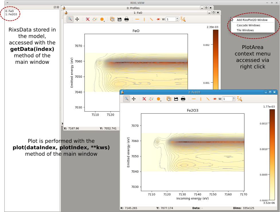
Figure 8.2.1 QtRIXS main window showing two RIXS data objects loaded in the model and plotted in the plot area.
Dock (= dragable) information widgets for selecting regions of interest on the plot and getting the coordinates can be added to the main window simply by:
main_win.addRixsDOIDockWidget(1)  #: the argument is the index of the plot
main_win.addRixsDOIDockWidget(2)  #: another info box for plot 2
The result is shown in Figure 8.2.2.
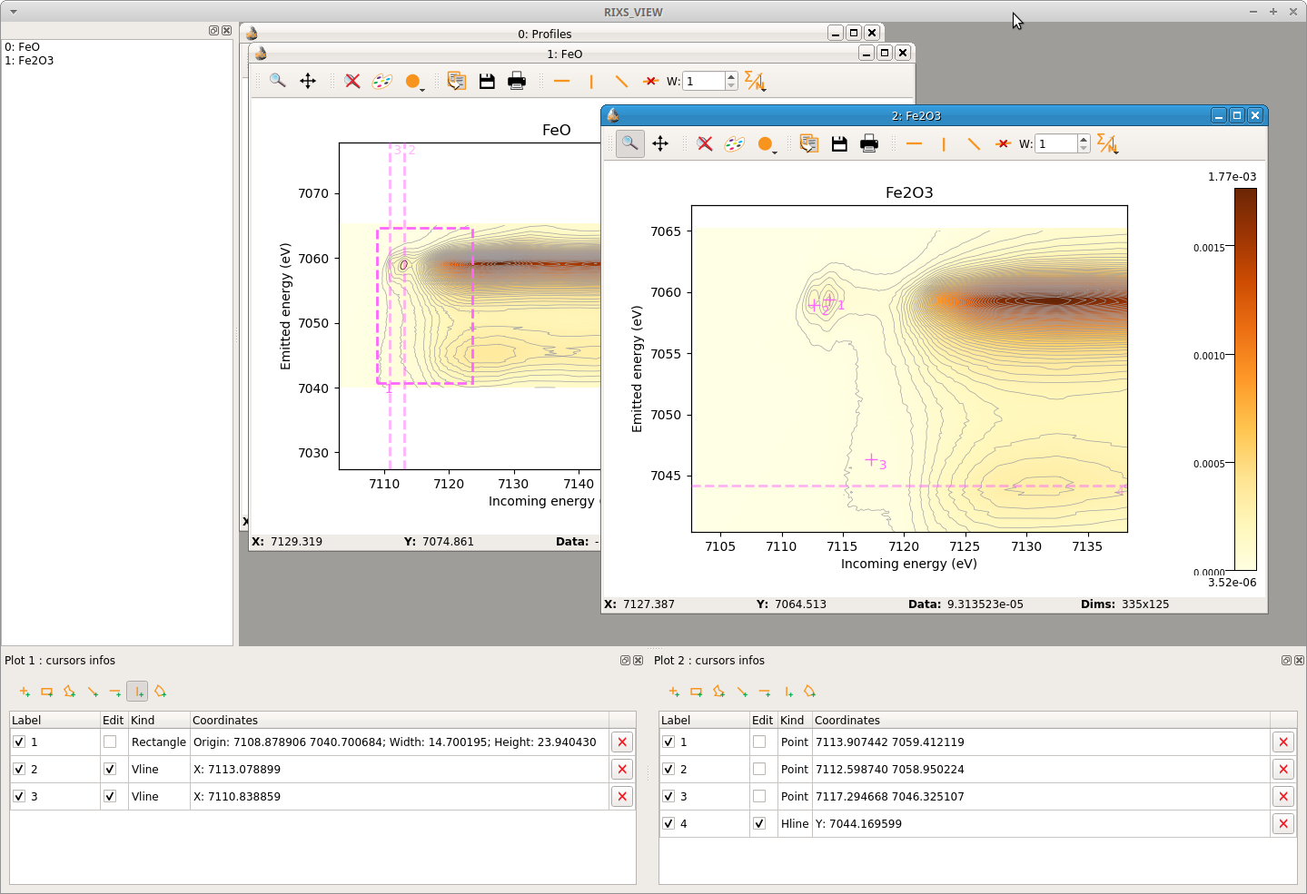
Figure 8.2.2 Main window with added two widgets for getting information on the regions of interest.
The data can also be cropped or plotted in energy transfer:
crop_area = (7108, 7040, 7120, 7065)
main_win.plot(0, 1, crop=crop_area, nlevels=10)  #: it is possible to change the number of contours lines for a better visualization
main_win.plot(1, 2, crop=crop_area, nlevels=10)
main_win.plot(1, 3, crop=crop_area, rixs_et=True, nlevels=10)
To take line cuts with a given width (in pixels), it is possible to use the toolbar on each RIXS plot. This will push the corresponding cut to a common plot window called Profiles. From that window is possible to save the profiles to ASCII files and then process them independently. The profiles toolbar works correctly for horizontal and vertical cuts only. For taking a diagonal cut in energy transfer (i.e., HERFD-XAS) the best is to simply take an horizontal cut in emitted energy. If the profiles window gets busy of many curves, the plot can be simply be cleaned by popping the context menu with right click on the legends. This is shown in Figure 8.2.3.
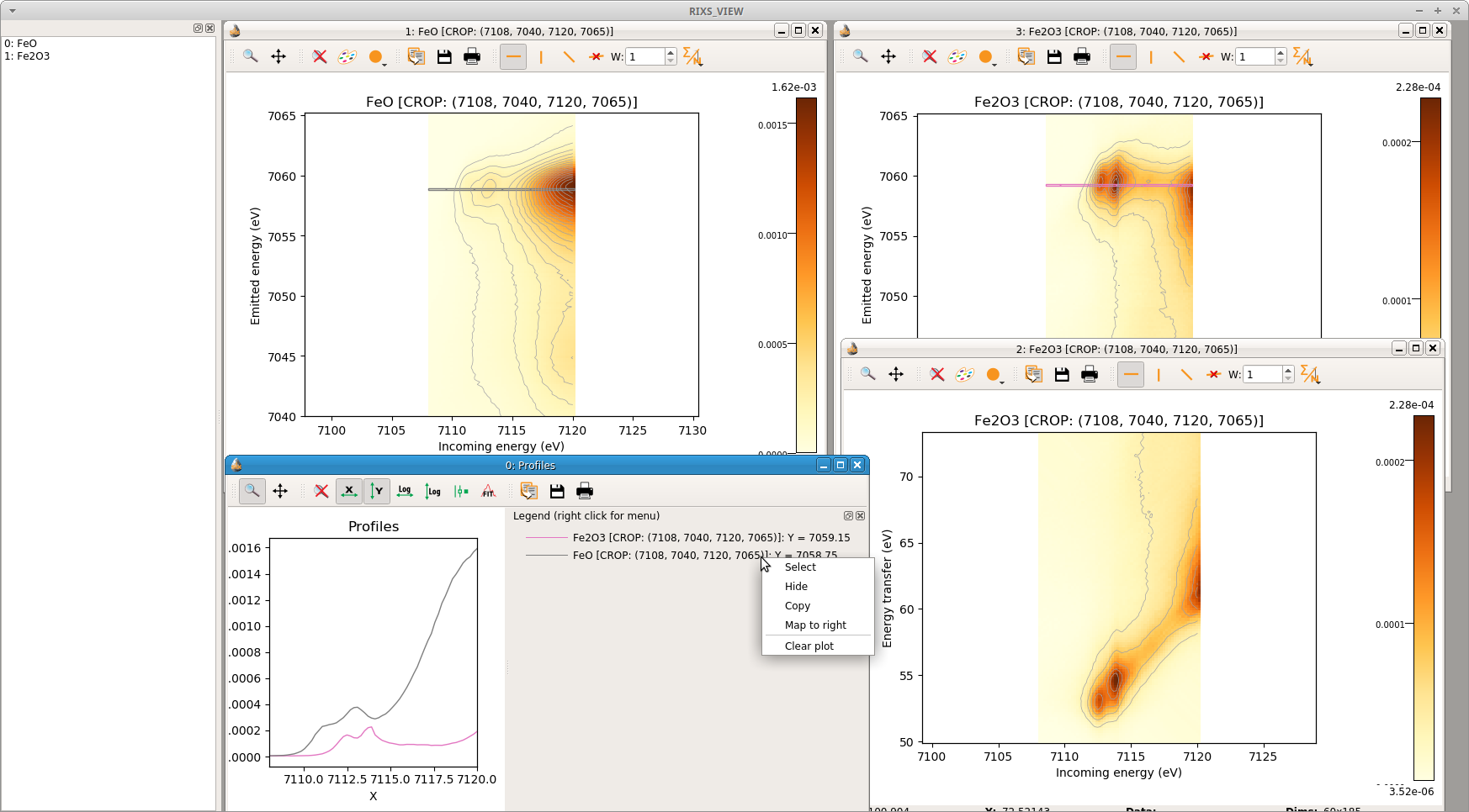
Figure 8.2.3 Cropped plots, plot in energy transfer and line cuts to visualize the profiles of the spectra. A context menu is available to clean, highlight or move one line to right axis of the plot.