4.3. XAS_Viewer

The XAS_Viewer GUI uses Larch to read and display XAFS spectra. This is still in active development, with more features planned with special emphasis on helping users with XANES analysis. Current features (as of March, 2018, Larch version 0.9.36) include:

• read XAFS spectra from simple data column files.
• read XAFS spectra from Athena Project files.
• XAFS pre-edge removal and normalization.
• visualization of normalization steps.
• fitting of pre-edge peaks.
• saving of data to Athena Project files.
• saving of data to CSV files.

The XAS Viewer GUI includes a simple form for basic pre-edge subtraction, normalization, and de-convolution of XAFS spectra. Figure 4.3.1 shows the main window for the XAS Viewer program. The left-hand portion contains a s list of files (or data groups) that have been read into the program. Clicking on the file or group name makes that “the current data group”, while checking the boxes next to each name will select multiple files or group. Buttons at the top of the list of files can be used to “Select All” or “Select None”.

The right-hand portion of the XAS Viewer window shows multiple forms for data processing, each on a separate Notebook tab. The main tab shown is labeled “XAS Normalization” with a form for normalizing XAS data, and choices for how to plot the data for the current group or the selected groups. This form is provides a graphical interface to the pre_edge() and related functions. A separate window (Figure 4.3.2) will show an interactive plot of the chosen data to be plotted. As with all Larch plots, the plot can be zoomed in an out, and configured to change colors, linestyles, text for labels, and so on. For example, clicking on the legend for each spectra will toggle the display of that spectra.

Note that many of the entries for numbers on the form panels have a button with a fancy ‘+’ sign. Clicking anywhere on the plot window will remember the energy value of the last point clicked. Then, clicking on one of these buttons will insert that “last-clicked energy” value into the corresponding field.

The XAS Viewer program has notebook tabs or more specialized XANES and XAFS analysis. Currently (March 2018), the only additional functionality is for fitting pre-edge peaks, which is under the “Pre-edge Peak Fit” tab as shown below, but we will be adding more functionality soon.

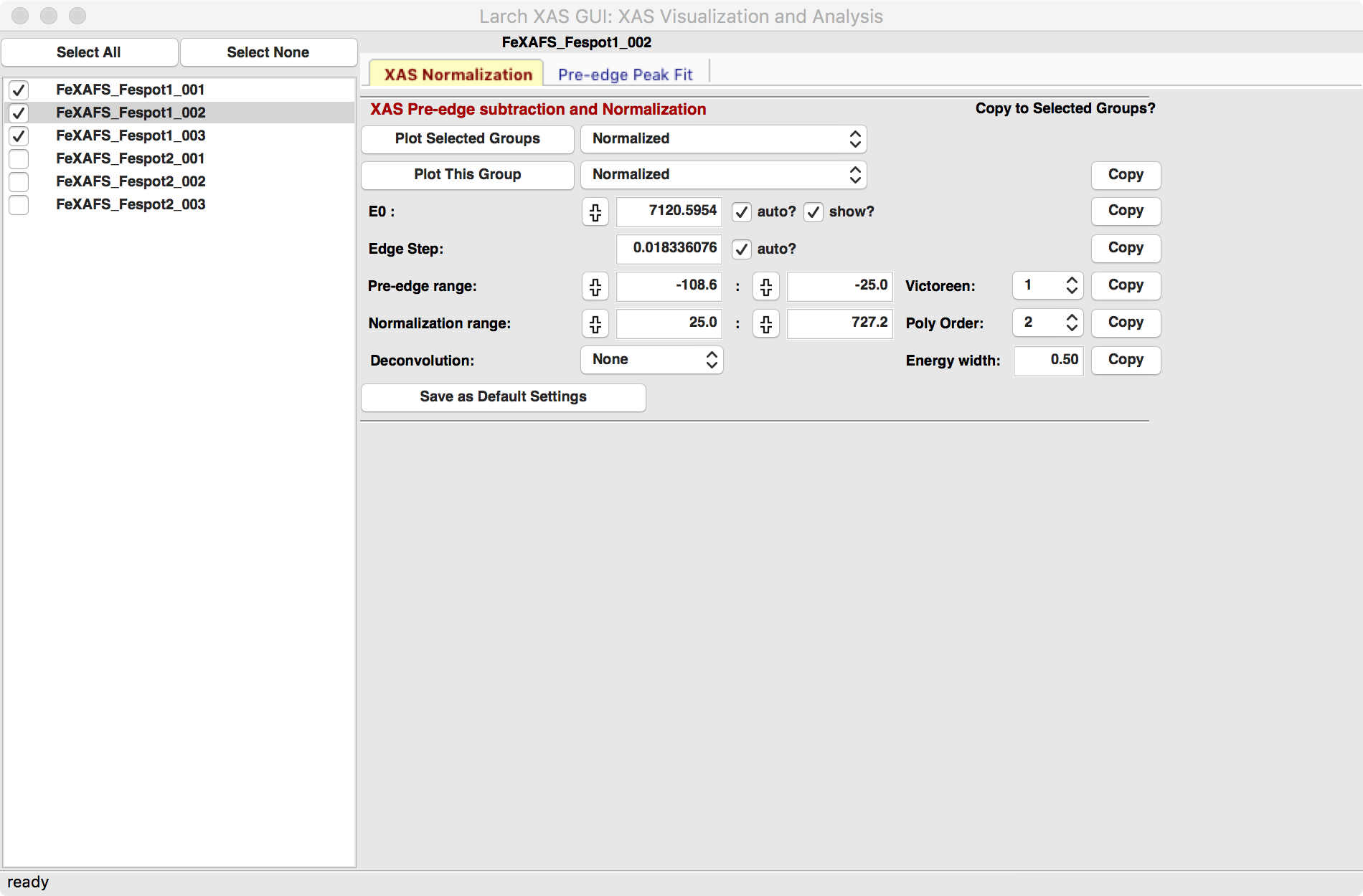
Figure 4.3.1 Main XAFS pre-edge subtraction and normalization form.

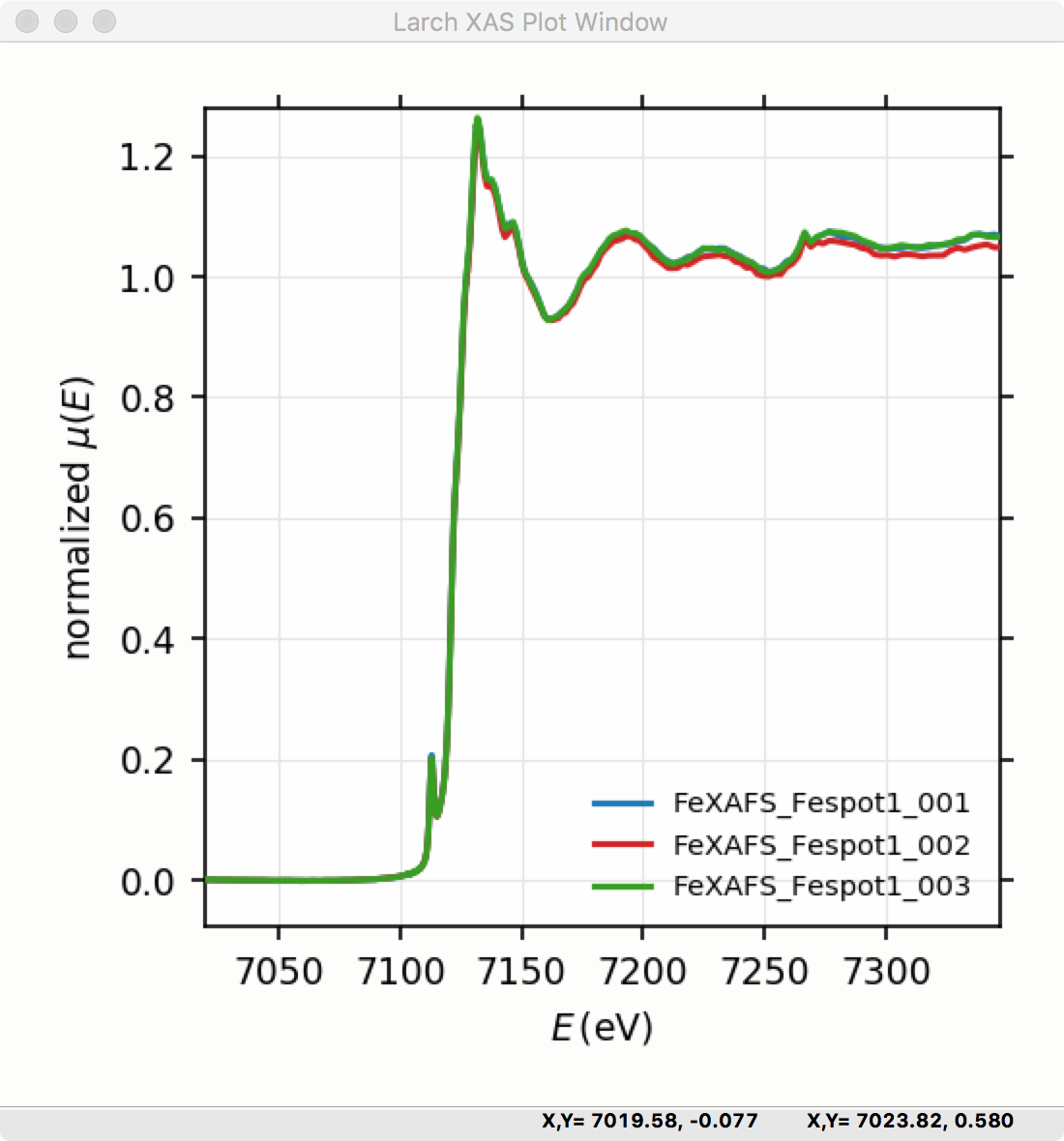
Figure 4.3.2 An example of an interactive plot of XANES data.

Data groups can be read from plain ASCII data files using a GUI form to help build \(\mu(E)\), or from Athena Project files, as shown in Figure 4.3.3 and Figure 4.3.4. Multiple data groups can be read in, compared, and merged. These datasets can then be exported to Athena Project files, or to CSV files.

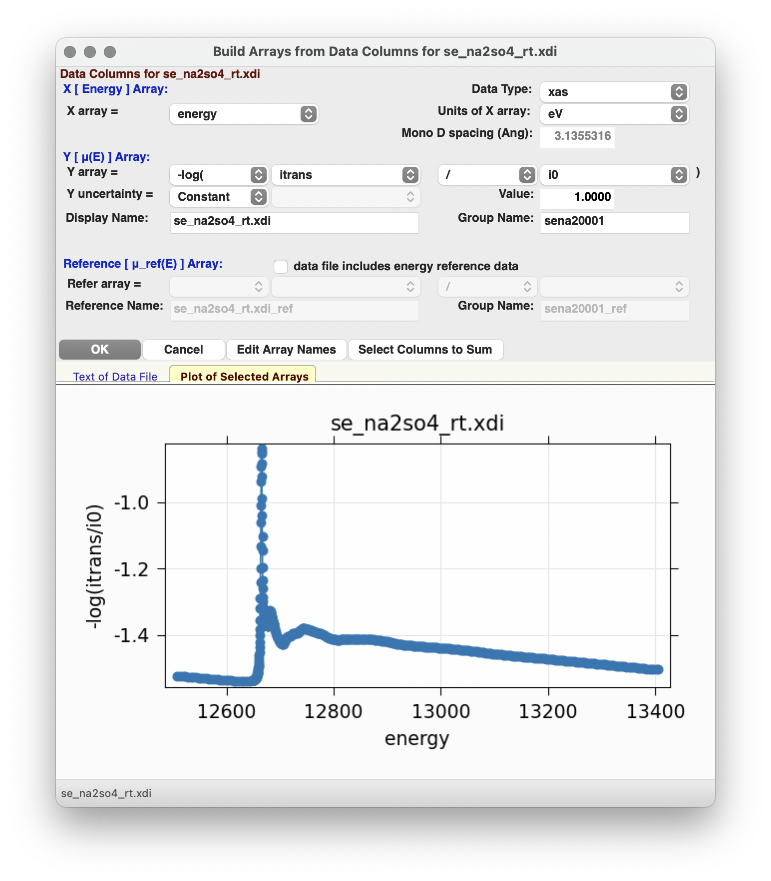
Figure 4.3.3 ASCII data file importer.

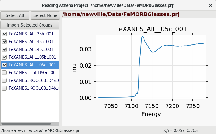
Figure 4.3.4 Athena Project importer.

The “Pre-edge Peak Fit” tab (show in Figure 4.3.5) provides a form for fitting pre-edge peaks to line shapes such as Gaussian, Lorentzian, or Voigt functions. This provides an easy-to-use wrapper around lmfit and the minimize() function for curve-fitting with the ability to constrain fitting Parameters.

To do fitting of pre-edge peaks with the interface, one begins by fitting a “baseline” to account for the main absorption edge. This baseline is modeled as a Lorentzian curve plus a line. Fitting a baseline requires identifying energy ranges for both the main spectrum to be fitted and the pre-edge peaks – the part of the spectrum where the baseline should not be fitted. This is illustrated in Figure 4.3.5 and Figure 4.3.6. Note that there are separate ranges for the “fit range” and the “pre-edge peak” range (illustrated with grey lines and blue ‘+’ signs on the plot). The “pre-edge peak” range should be inside the fit range.

Clicking “Fit baseline” will fit a baseline function and display the results. The initial fit may have poorly guessed ranges for the pre-edge peaks and fit range and may require some adjustment.

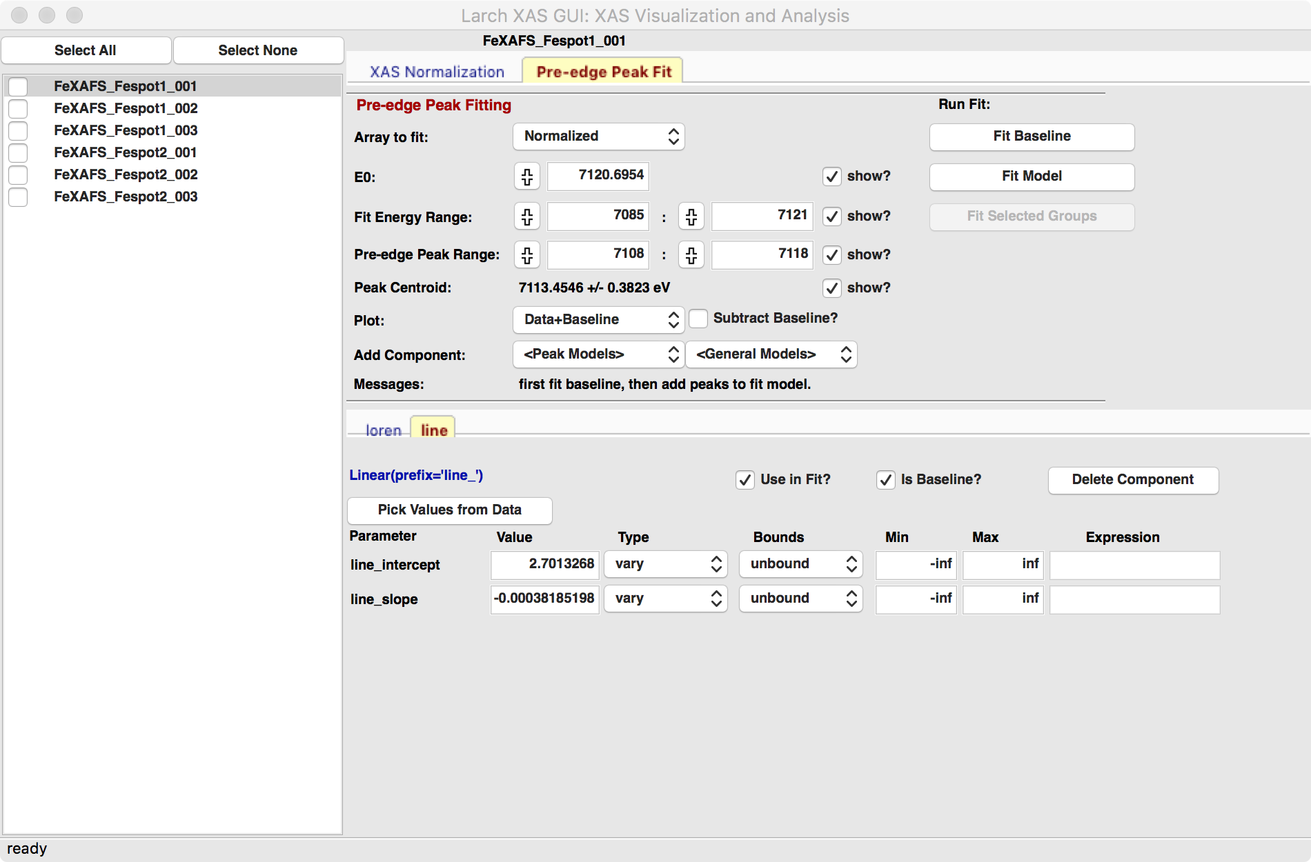
Figure 4.3.5 Pre-edge peak Window of XAS_Viewer, showing how select regions of pre-edge peaks for fitting a baseline.

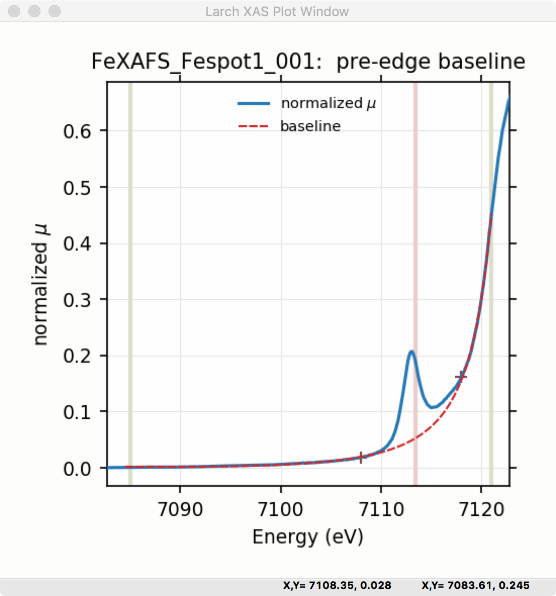
Figure 4.3.6 Plot of pre-edge peaks with baseline. Note that the grey vertical lines show the fit range, the blue crosses show the pre-edge peak range, and the pink line shows the centroid of the pre-edge peaks after removal of the baseline.

Once the pre-edge baseline is satisfactory, you can add functions to model the pre-edge peaks themselves. Select one of the “Peak Models” (typically Gaussian, Lorentzian, or Voigt), which will show a new tab in the “model components area” in the lower part of the form. Note that the baseline will consist of a Lorentzian and linear model component, so that there will be at least 3 tabs for the 3 or more components of the pre-edge peak model. This is shown in Figure 4.3.7, which shows the form for 1 Gaussian peak, and the baseline. You can include multiple peaks by repeatedly selecting the peak type from the drop-down menu.

After selecting a peak type, click on the “Pick Values from Data” button, and then pick two points on the plot to help give initial ranges for that peak. The points you pick do not have to be very accurate, and the initial values selected for the amplitude, center, and sigma parameters can be modified. Note that you can place bounds on any of these parameters – it is probably a good idea to enforce the amplitude and sigma to be positive. If using multiple peaks, it is often helpful to give realistic energy bounds for the center of each peak, so that they do not overlap.

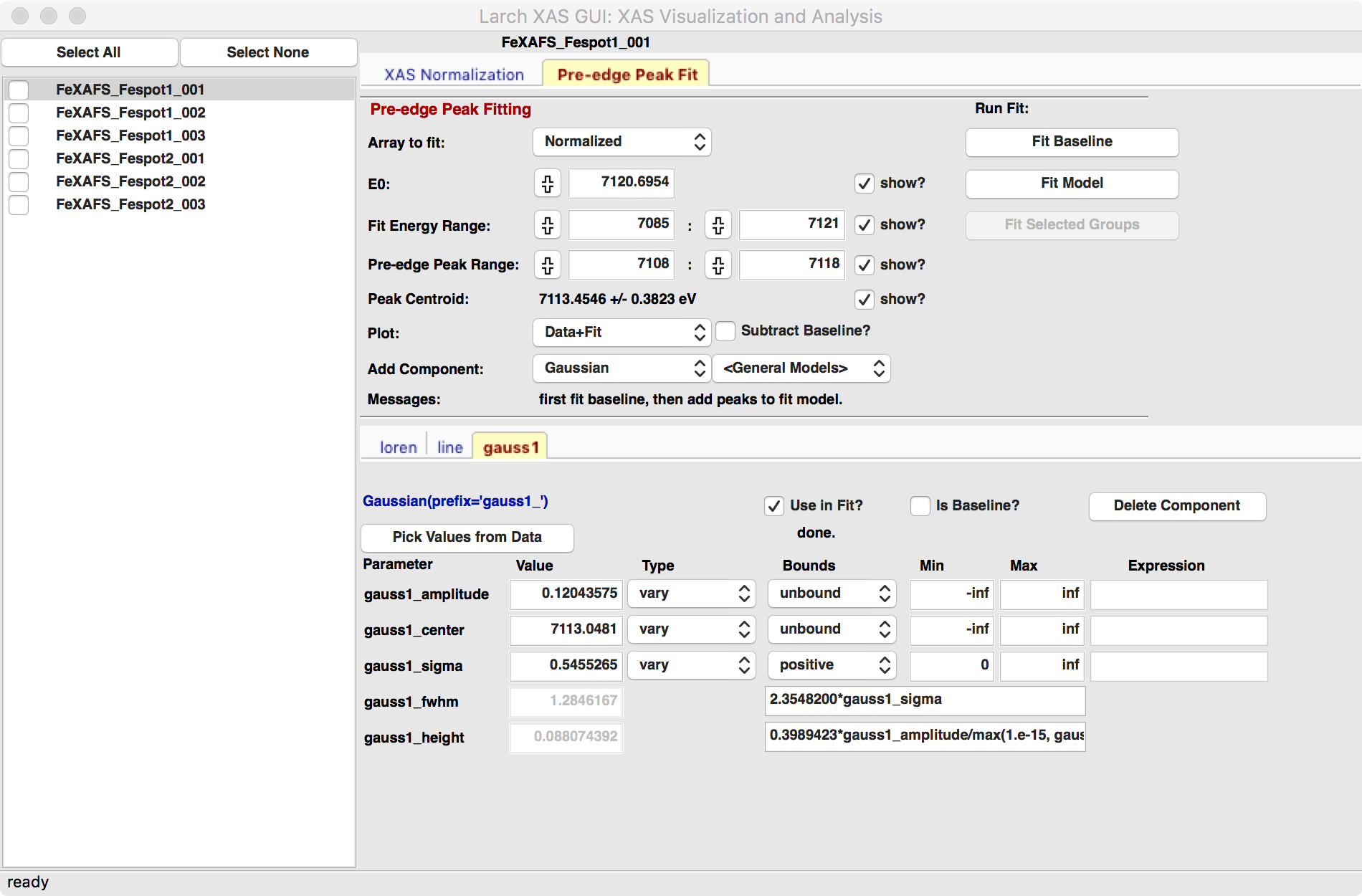
Figure 4.3.7 Pre-edge peak Window of XAS_Viewer, showing how select regions of pre-edge peaks for fitting a baseline.

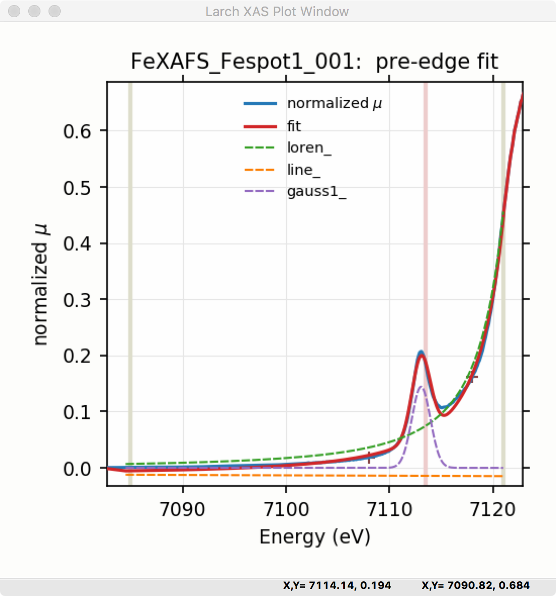
Figure 4.3.8 Pre-edge peak Window of XAS_Viewer, showing how select regions of pre-edge peaks for fitting a baseline.

Upon doing a fit, the plot is updated to show the data, best-fit, and each of the components used in the fit (Figure 4.3.8). Fit statistics and best-fit parameter values, their uncertainties, and correlations are shown as a report in a separate window, with an example shown in Figure 4.3.9. Note that for peaks such as Gaussian, Lorentzian, and Voigt, not only are amplitude (that is, area under the peak), sigma, and center shown but so are fwhm (full width of peak at half the maximum height) and height (the maximum height of the peak).

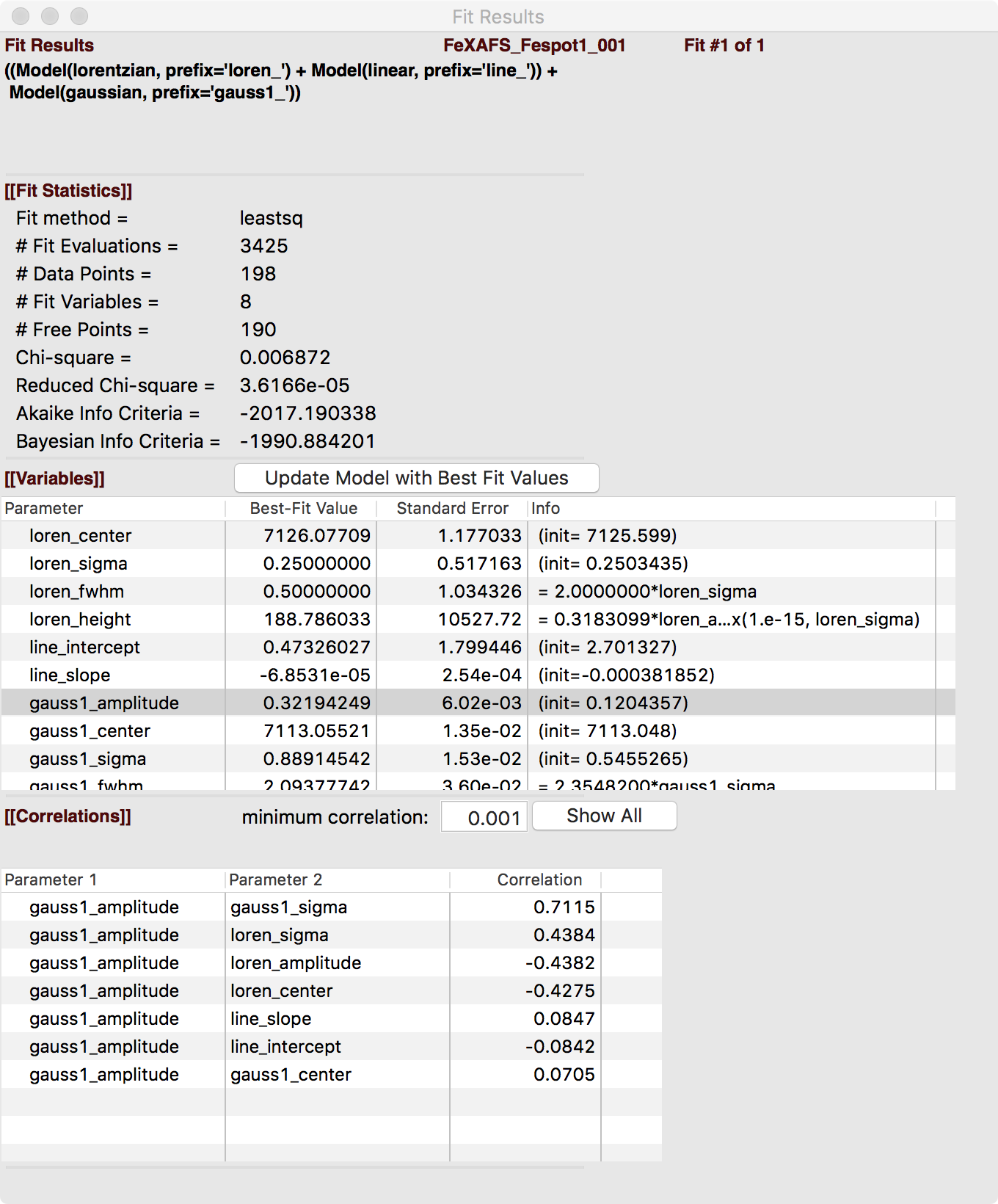
Figure 4.3.9 Fit result frame for Pre-edge peak fit.

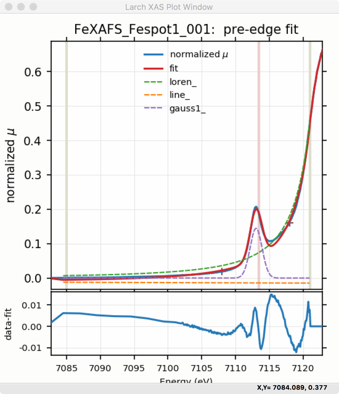
Figure 4.3.10 Pre-edge Peak fit with residual.

Though the plot of the fit in Figure 4.3.8 looks good, plotting the fit along with the residual (by selecting “Data+Residual” in the drop-down menu of “Plot:” choices) as shown in Figure 4.3.10 reveals a systematic mis-fit. That is, the data-fit for this model clearly shows some spectral structure beyond just the noise in the data. Adding a second Gaussian (and maybe even a third) will greatly help this fit. To do that, add another Gaussian peak component to the fit model using the drop-down menu of “Add component:”, select initial values for that Gaussian, and re-fit the model. We’ll leave that as an exercise for the reader.

Fit results can be saved in two different ways, using the “PreEdge Peaks” menu. First, the model to set up the fit can be saved to a .modl file and then re-read later and used for other fits. This model file can also be read in and used with the lmfit python module for complete scripting control. Secondly, a fit can be exported to an ASCII file that will include the text of the fit report and columns including data, best-fit, and each of the components of the model.